By: Brett Stoddard
Background
Thermal sap flux (or flow) sensors have been popular amongst environmental sensing experts since the mid-20th century. They measure the velocity of sap through the stem or trunk of a plant using an array of heaters and temperature sensors.
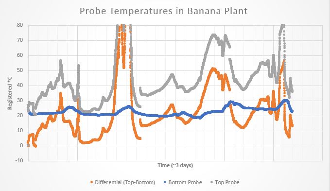
A modern sap flow variant, proposed by Grainer, is made up of two temperature sensing probes directly above and below a heater probe—all spaced evenly. When a measurement is taken, the heater probe turns on and emits a heat pulse for several seconds. Then the temperature difference between the upper and lower probe is recorded. The temperature difference over time can be used to track sap flow (the specifics of this will be talked about in a later blog post).
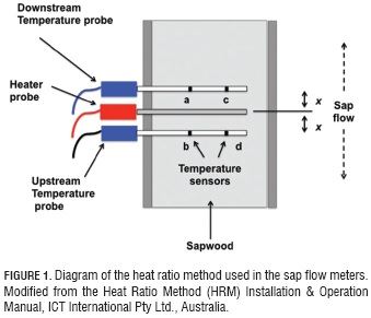
Figure from paper by Bayona-Rodríguez et al (2016)
Goal
To construct a sap flux sensor using surface mount technology (SMT) which can be manufactured using an entirely automated setup given a pick-and-place machine but can still be made by hand by a person with adept soldering skills.
Challenges
The biggest challenge for this project is minimizing the width of the probes. Inserting any foreign object into the xylem of any plant will alter how sap flows through it. As such, minimizing the size of the probe is critical to accurate measurements. Current commercial probes have diameters of around 1.5mm (http://dynamax.com/products/transpiration-sap-flow/tdp-sap-velocity-thermal-dissipation-probe).
Limitations in commercial PCB etching process are a limiting factor in the minimum size of these probes. Also, if a sufficiently small probe size is achieved, the number of plant types this can be used on increases. For example, a large probe may only be used on trees of a sufficient diameter while a smaller one could be used on crops such as corn.
Method
To design the PCB designs for sap flow probes, Eagle CAD was used. Sparkfun has a solid tutorial on learning the basics of PCB design (https://learn.sparkfun.com/tutorials/using-eagle-schematic). OSHPARK is a popular PCB vendor that is easy to order from and so their DRC was used for this project (http://docs.oshpark.com/design-tools/eagle/design-rules-files/). Using these limitations, a PCB probe diameter of ~2.5 mm was achieved.
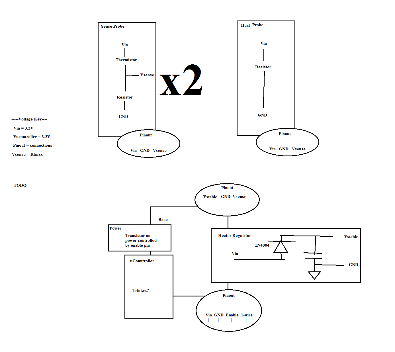
For the temperature sensor probe thermistors were chosen to be the sensor component. Thermistors were chosen because of their high level of sensitivity when compared to other sensors. Thermistors act as variable resistors that alter their resistance based on their temperature. The main drawback to using thermistors is that their output is not linear, but rather follows a logarithmic curve and so they are difficult to work with. For this probe, a voltage ladder was used to retrieve the resistance of the thermistor as shown in the schematic in the results section.
The heater element consists of a 50 ohm, US0603 footprint resistor with a 0.38 wattage rating. A future blog post will go more in-depth on how the resistance was calculated.
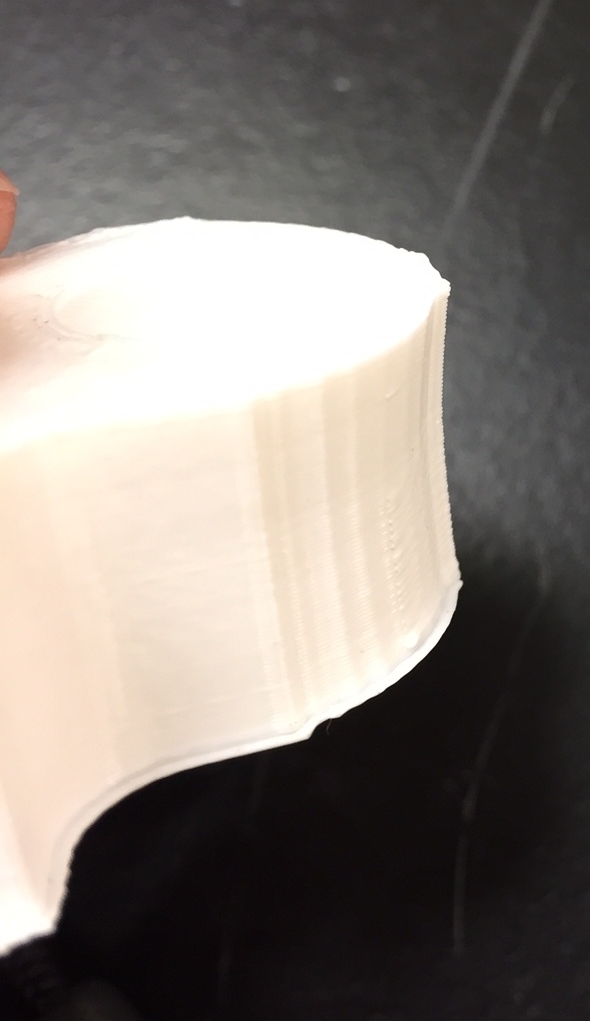
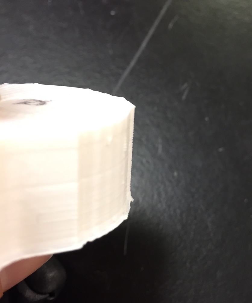
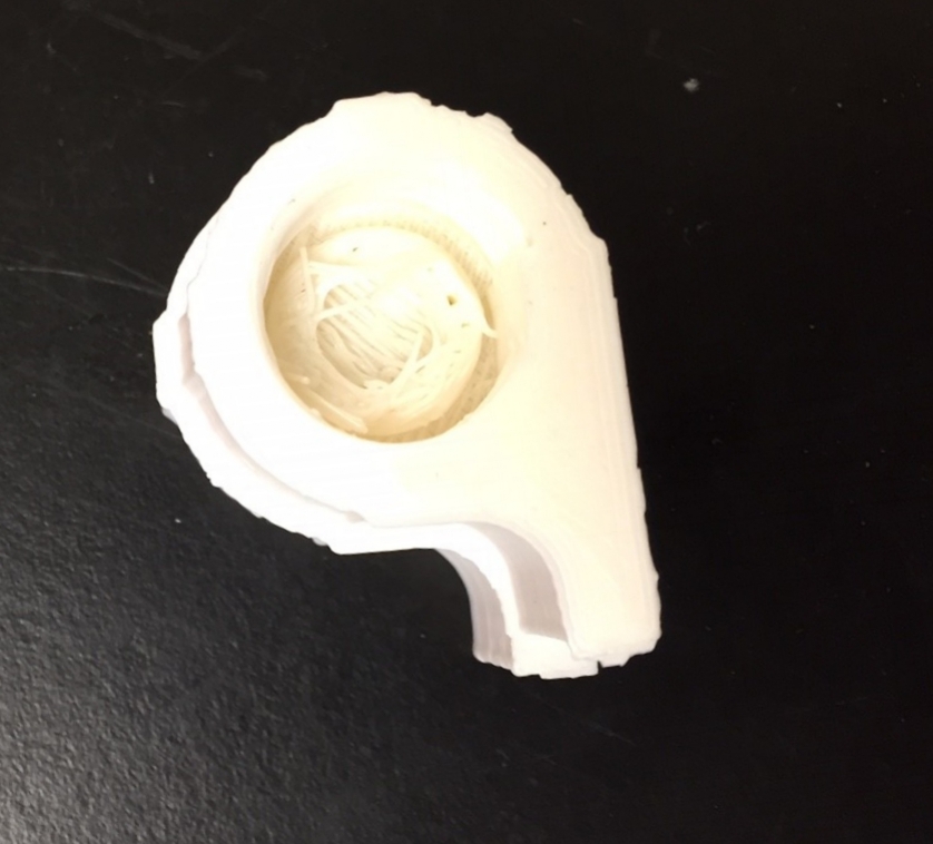
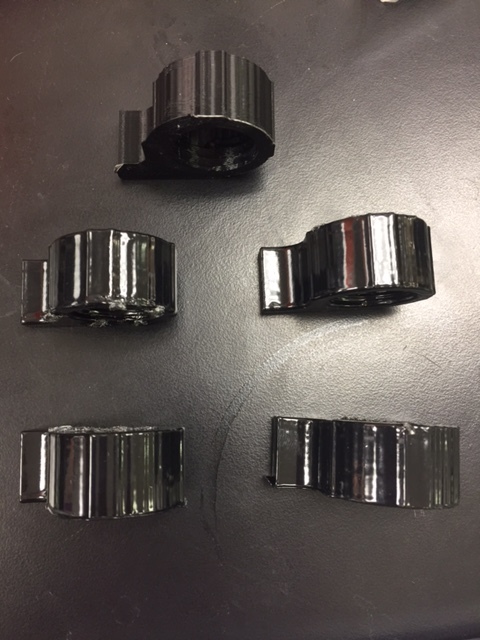
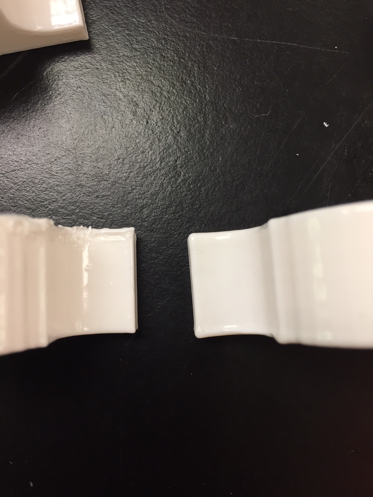
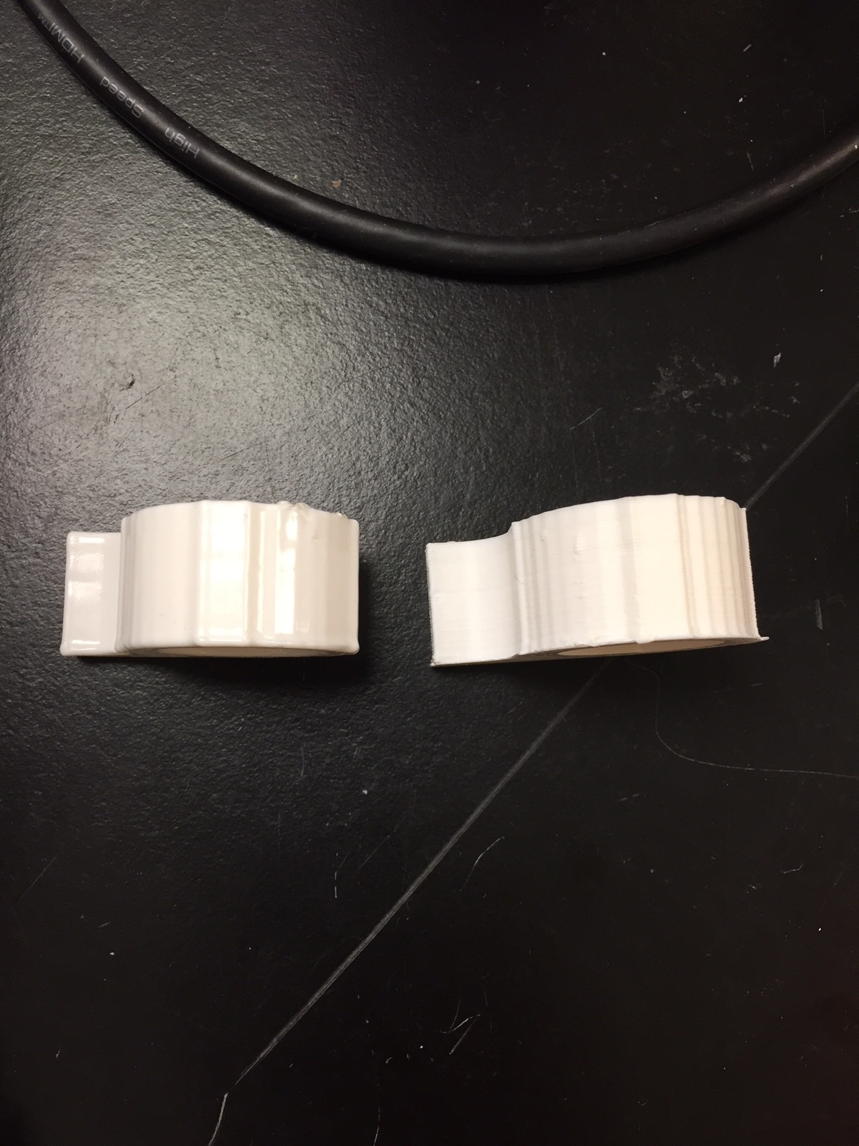
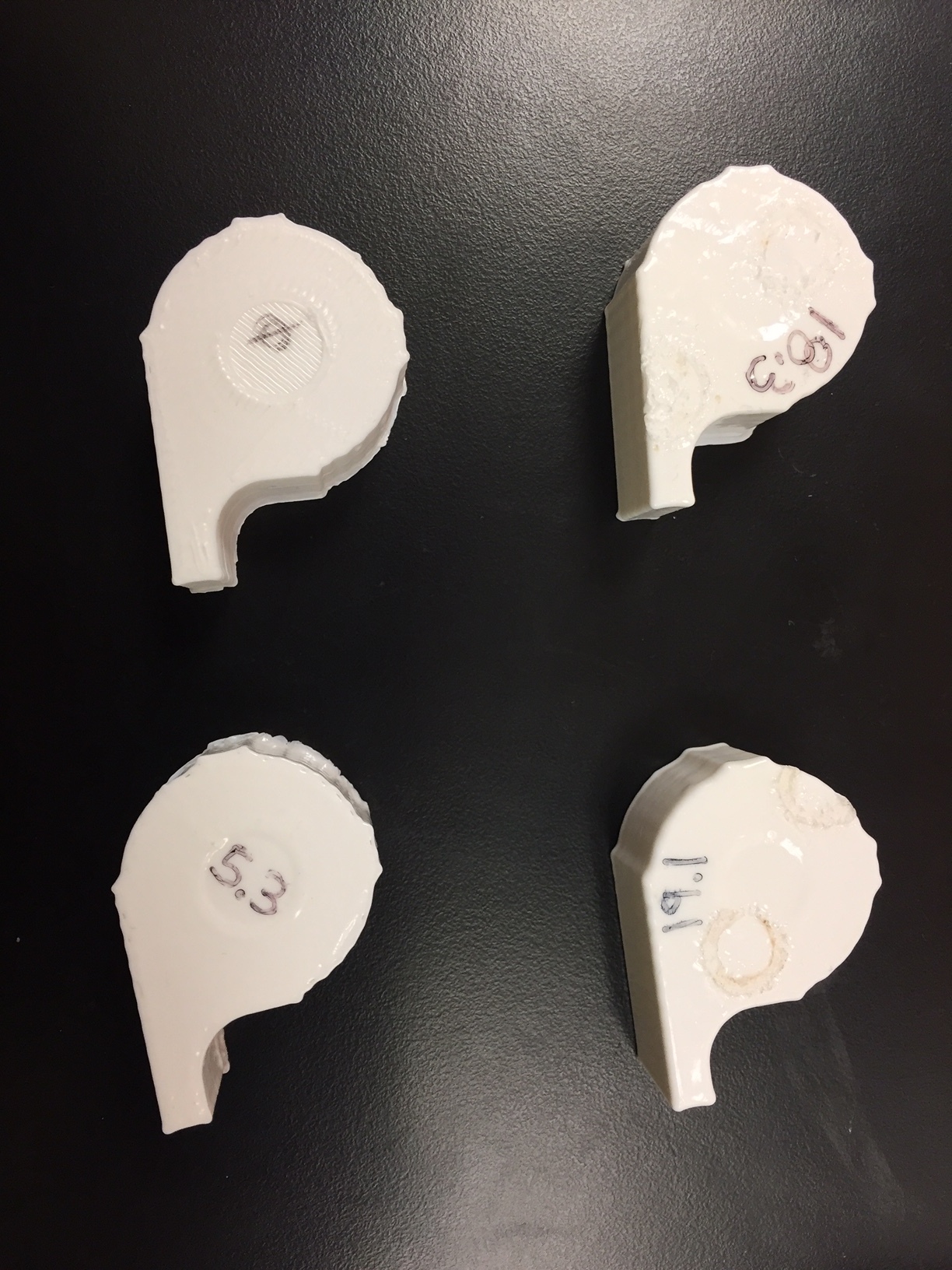
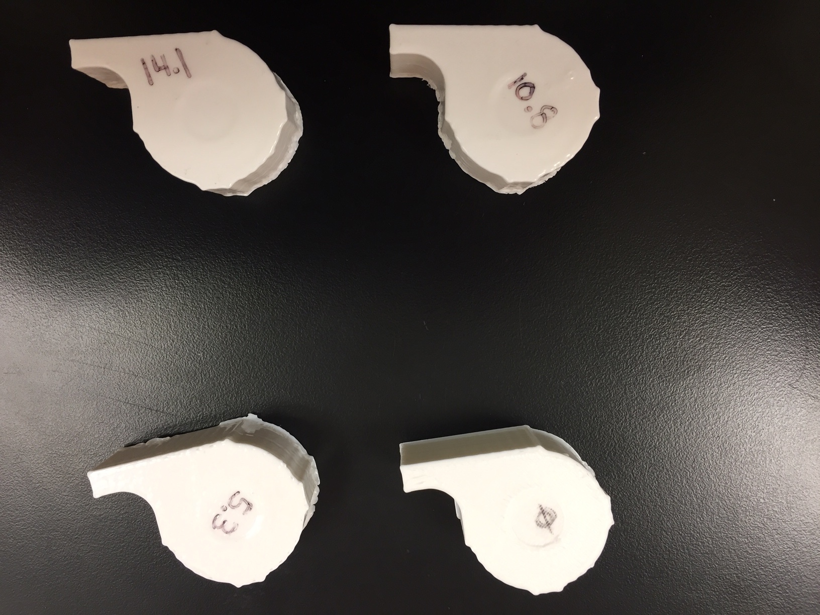
To maximize contact with the plant’s xylem, thermal epoxy was used in a mold around all three PCB probes. This was designed in SolidWorks 2017 and printed on a FormLabs Form 2 SLA printer for maximum resolution. The inside of this mold was coated in mold release spray to prevent the thermal epoxy from sticking to it. After the epoxy was sufficiently dried, a layer of silicone conformal coating was applied to waterproof each of the probes.
To control the sensor, a microcontroller with built-in ADC’s (here an Adafruit M0 Trinket) was used. The output pins on the temperature sensors were connected to the analog inputs of the microcontroller. An NPN transistor sat between a voltage source and the heater and was controlled by an output pin on the microcontroller.
Results
Images of the final PCB are shown below. It uses standard US0603 footprint resistors.
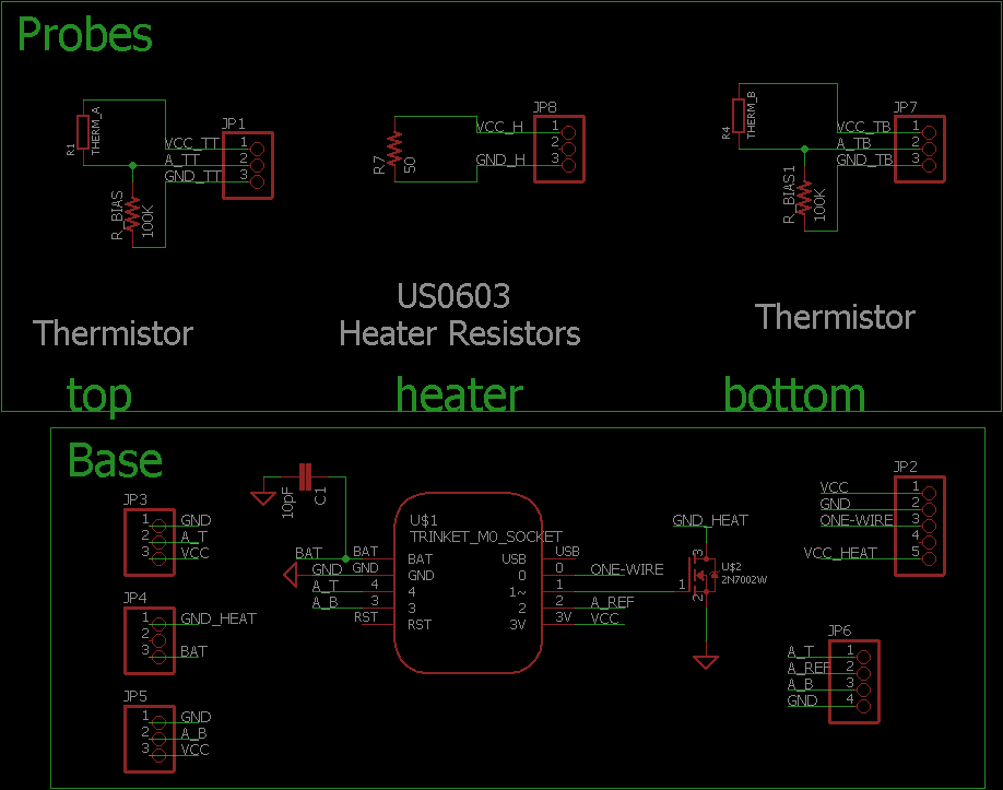
Schematic of the Sap Flow/Flux sensor with thermistor temperature sensors.
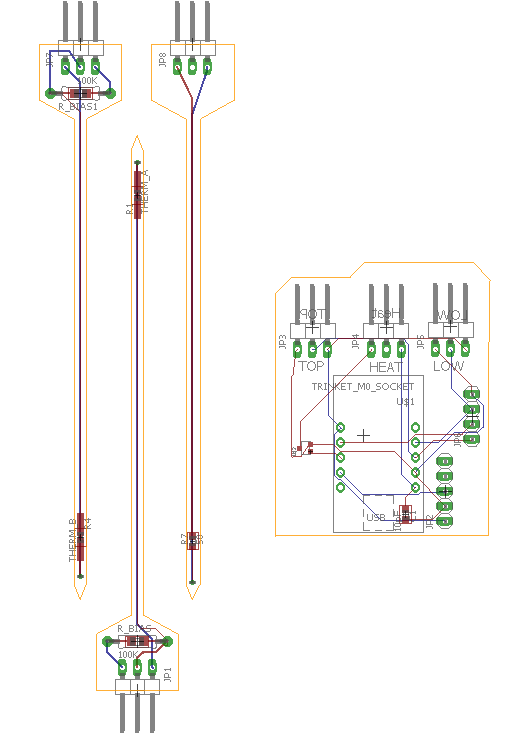
Image of the board design for Sap Flow sensor with thermistor temperature sensors. The two probes on the left are the thermistors and the one on the right is the heater probe. The PCB on the right houses an Adafruit M0 Trinket.
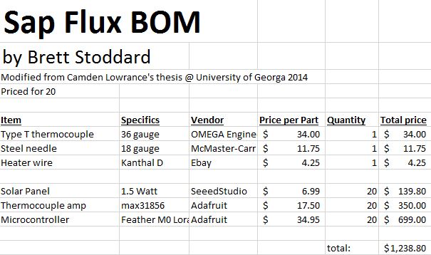
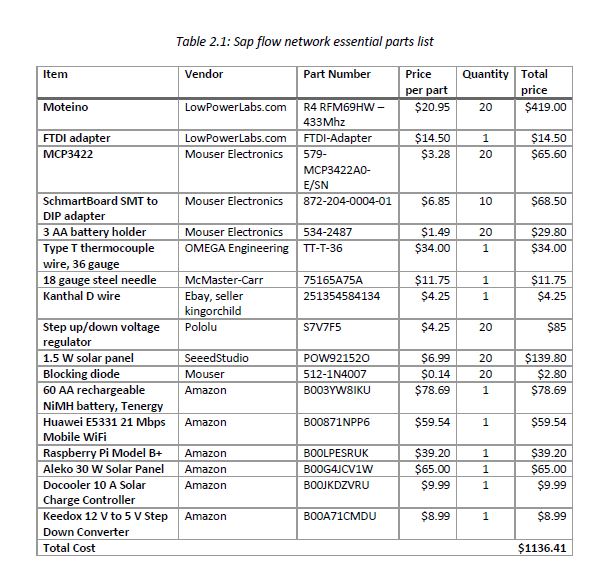
The bill of materials used is below.
A future blog post will go into a more detailed, step-by-step tutorial on how to build your own! It will also have finalized design files and best pracitces.
Room for Improvement
As with any project design, there are a multitude of ways that this could be improved. A few ideas with good potential are listed below in no particular order:
- Linearizing voltage output using a parallel thermistor configuration
- A/D conversion on the probe sensor to avoid signal loss across the line
- Housing to protect the temperature probes from solar radiation
- Insulation to protect the probes from ambient temperature fluxes
References
In order that they appear:
- Dynamax TDR Probes http://dynamax.com/products/transpiration-sap-flow/tdp-sap-velocity-thermal-dissipation-probe
- Sparkfun Eagle Tutorial https://learn.sparkfun.com/tutorials/using-eagle-schematic
- OSHPARK DRC for Eagle http://docs.oshpark.com/design-tools/eagle/design-rules-files/
External Links
In no particular order:
- Adafruit 12 bit ADC forum post
- Feather Lora RFM95 Adafruit tutorial
- Evaporimeter blog