The CO2 and luminosity sensors are transmitting data from one Feather M0 to another via OPEnS’ Nordic transmitter. Data is also saving locally with RTC time stamp to an Adalogger SD card.
A temporary voltage divider circuit was created with resistors to knock the K30’s data lines down from 5V to 3.3V for the Feather. A logic level shifter (https://www.sparkfun.com/products/12009) is on its way for the proper setup.
I’ll work on getting everything up on the GitHub page including wiring.
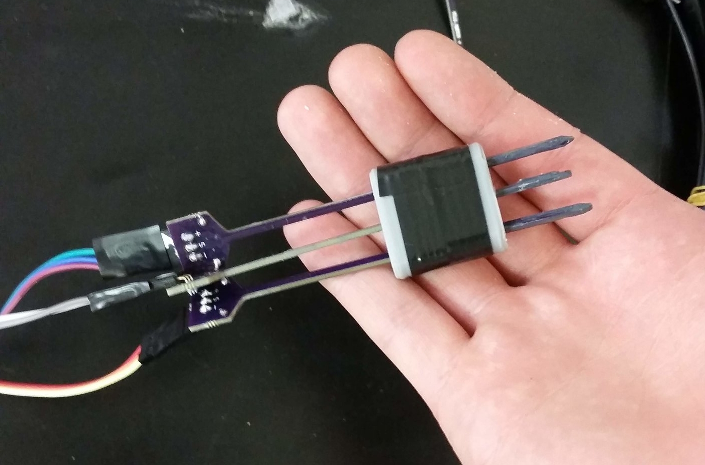
A probe was built as described in this build-guide. The following data was returned from the sensor.
Methods
An Adafruit Feather M0 with Lora capabilities was used to take measurements from the sap flow sensor. It activated an NPN mosfet that was connected in series with the +battery the heater probe and ground (or -battery).
Analog values were recorded by the board’s dedicated analog in pins. As per default, these readings were 10-bit although the M0 chip has the capability to do 12-bit ADC (detailed in this link). This would increase the theoretical precision four-fold and is something that should be investigated in the future. These raw values were logged onto an SD card. The electronics were run off of a 4AH battery until it died (after around days).
Additionally, an Adafruit SHT31-D breakout board was wired up and placed in the enclosure to provide ambient temperature values that also recorded day-night cycles.
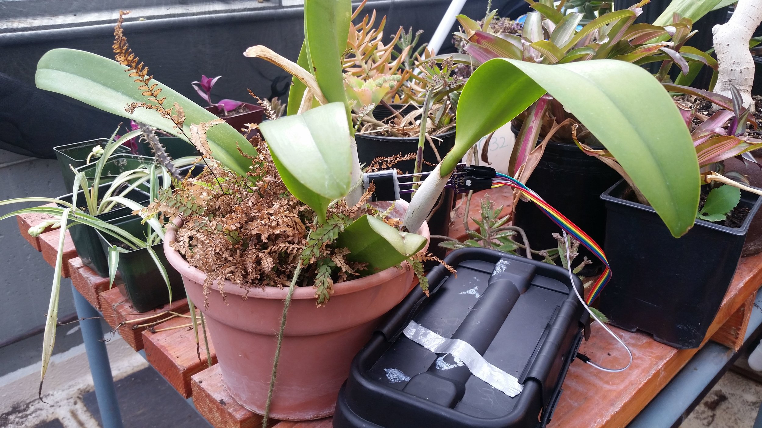
In order to make the setup water resistant, electrical tape was wound around any electrical connections, the probes were covered in silicone conformal coating, and the microcontroller and battery were placed in a waterproof box, the DriBox.
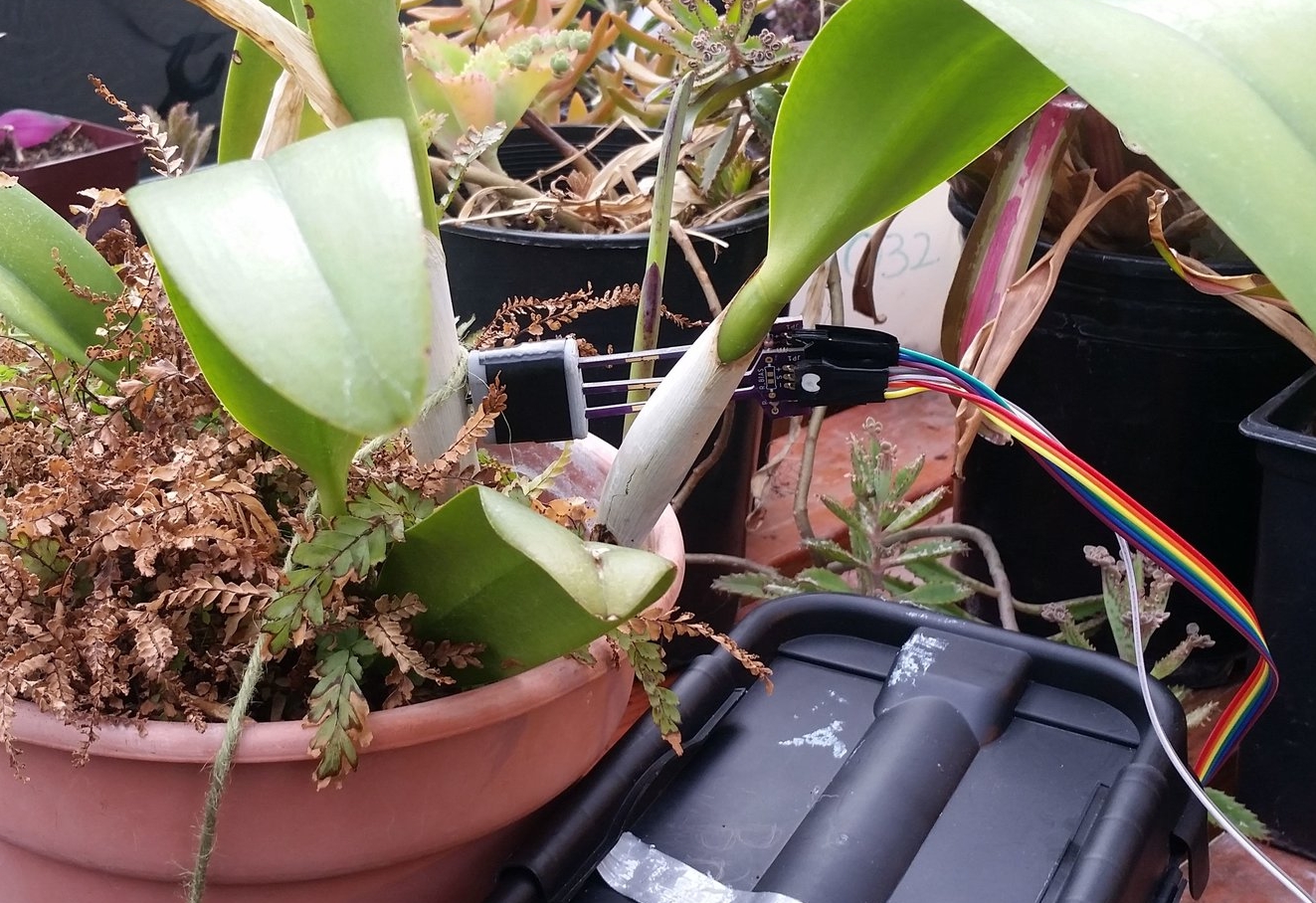
Image of the testing setup.
Results
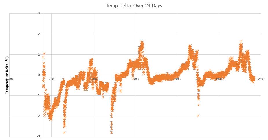
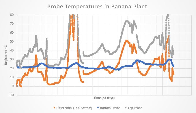
The following graph was determined from the plant data. As you can see, there is a cyclic pattern happening, with the temperature differential. However, there are also several large “spikes” in the data. Talking with the greenhouse manager, it turns out that the timing of those spikes corresponds directly with the time he waters the plants. Best guest, water either cooled down one of the probes or got into the connections and acted as a short briefly before evaporating. The full raw data can be downloaded here.
Graph over ~3.6 days worth of data. Data was logged every 60 seconds by an Adafruit M0 Feather with Lora.
To determine the exact temperatures from the two probes, two equations were used. The first one was a simple voltage divider equation to get the resistance of the thermistor. From the resistance, the thermistor beta equation was used to determine the temperature. The beta value for the beta value of the thermistor used (link here) was determined from its product datasheet. Unfortunately, the exact equations used were removed when I saved the file as its native CSV format after editing it in excel instead of saving it in an excel format (learn from my mistakes!).
This post will provide step by step instructions on how to build your own thermal dissipation sap flow sensor. Seperate blog posts fully explain the what a thermal pulse sap flow sensor does, the idea behind this design, and the code involved (coming later).
A probe in the hand is worth two in the bush. Probes are not angled correctly in this image.
Index
Order parts
Solder probes
Apply thermal epoxy
Wire it up
Program microcontroller
Install in a plant.
Step 0: Required Tools
Before jumping into the project, it’s important to mention that this project requires a few specialty devices to make.
The Feather M0 can be substituted for any micro controller with analog-in pins with some changes to the code to accommodate these new pins (mentioned briefly in Step 4) and if a different voltage batter is used, you should take a look at this blog post and change the heater resistor value.
When ordering the electronic parts I would highly suggest you buy spare parts, especially any 0603 resistors (I baked those into the single sensor BOM). It’s important to note the tolerance of the bias resistor (line 5), a lower tolerance can be used if it is calibrated for (a later blog post should talk about this).
Step 2: Solder Probes
Once you’ve received all the parts, it’s time to break out the soldering iron, tweezers, and reading glasses (optional) to tackle the most difficult step of this build: soldering on US0603 sized resistors. Soldering these on is a major test of patience even for veteran electrical engineers, but not impossible for first-time solders. Here are a few tips and tricks that should help: article from build-electronic-circuits.com, video from Engenuics Technologies.
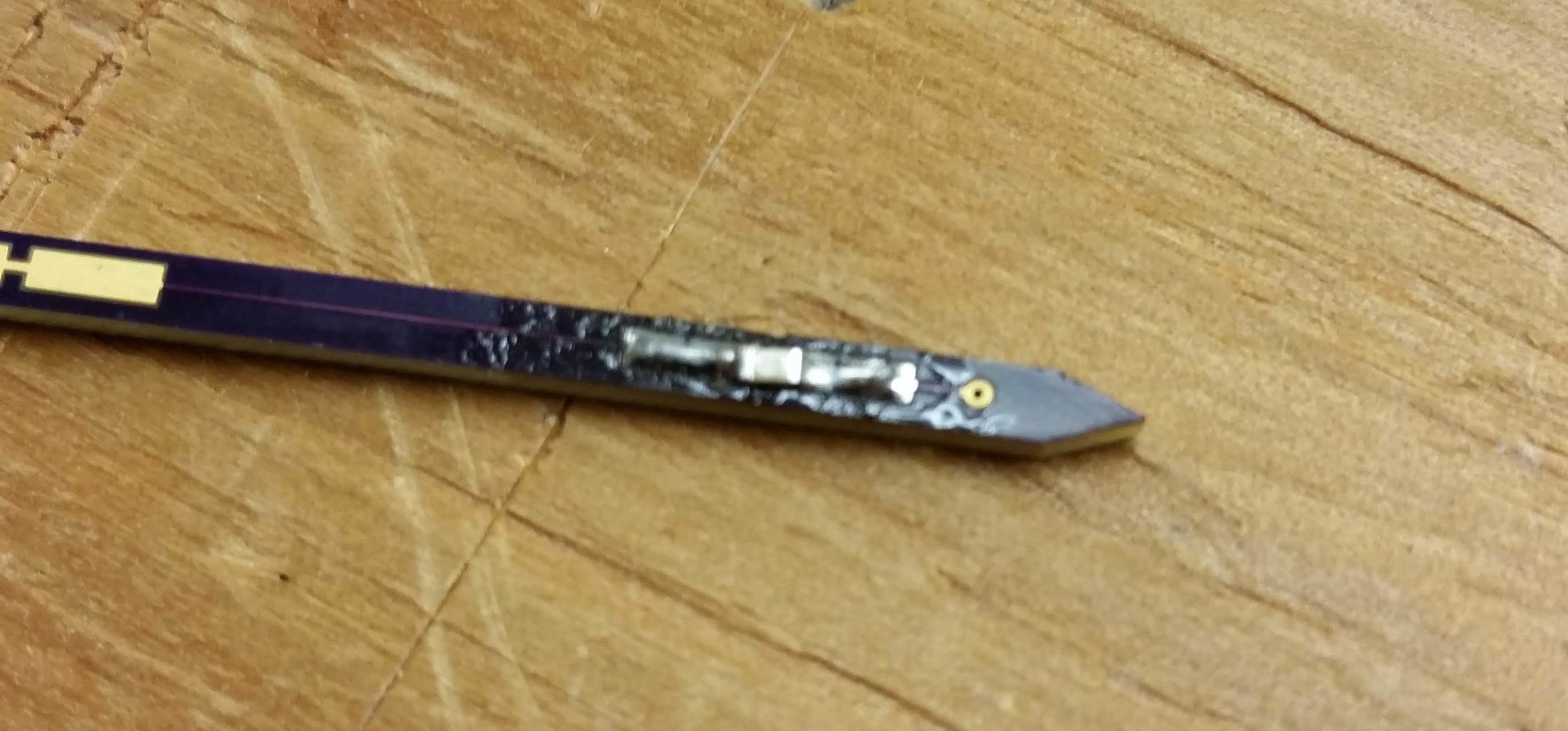
Thermistor properly soldered on the end of a probe. These suckers are TINY!
For the current design, three resistors need to be soldered: two thermistors and one low-ohm heater resistor. I find it helpful to mark which one is which immediately after soldering with some nail polish so I don’t get them confused because they look identical.
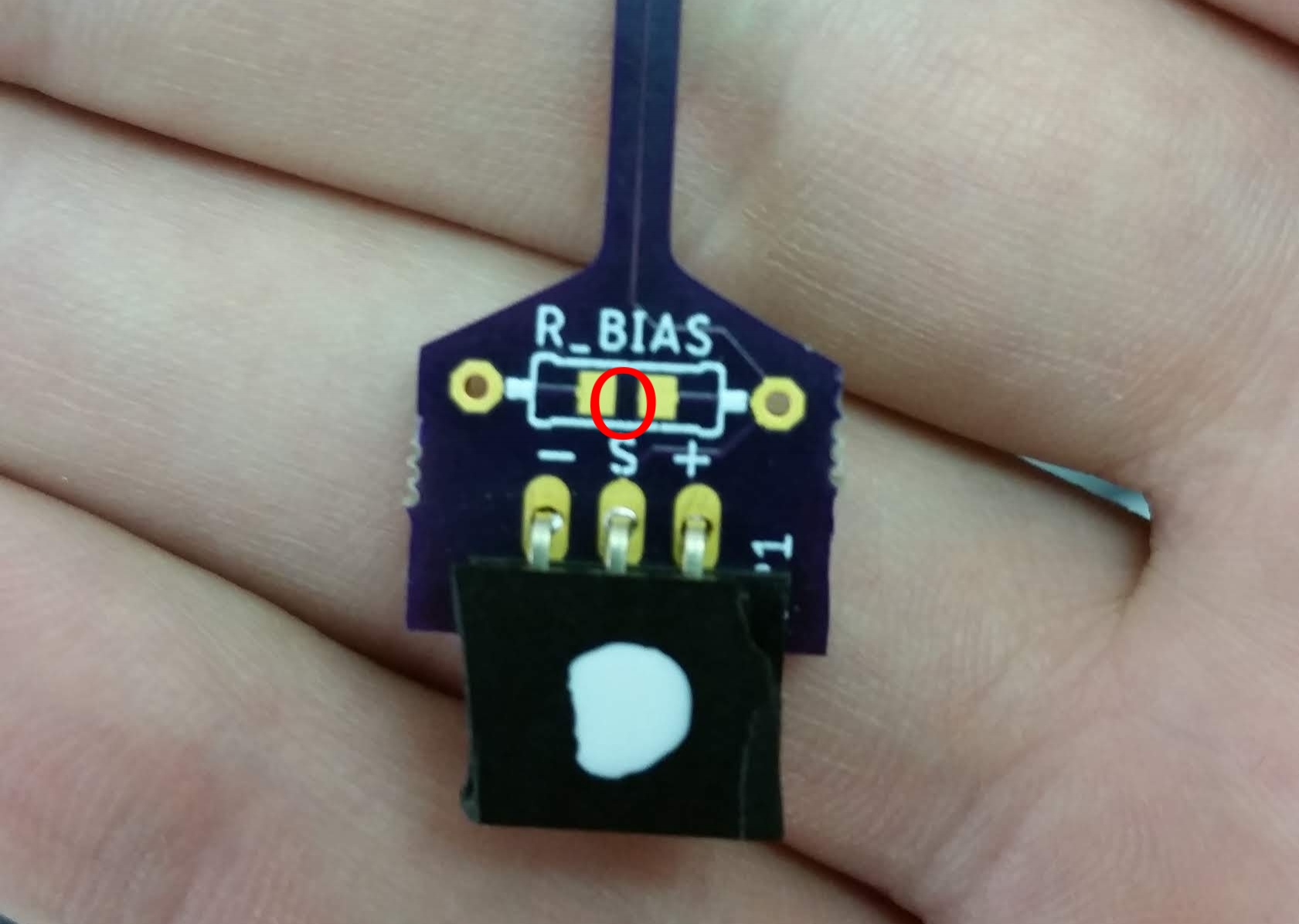
After the tiny resistors are in place on the end of the probe, its time to move down and solder on connectors on all the probes, 100K ohm bias resistors on the thermistor probes, and “short” the bias resistor on the heater probes using a large clump of solder on the 0603 pads (circled in red below). Use a multimeter to make sure all solder points are good and that the probe resistor is not shorted. The temperature probe should have a resistance of ~100k (this will vary based on temperature). The heater probe should have a resistance of 50 ohms (or whatever heater ohm is chosen).
Image of the base of the heater resistor. Notice the 90 deg female headers, the dip of fingernail polish identifying it, and the lack of a bias resistor. Probes with the thermistor will have a bias resistor. The bias resistor has optional pads to replace the through-hole mount with another 0603 resistors cirlced in red– for the heater probes these should be “shorted” using a large glob of solder.
As kind of a placeholder, the current connectors on the probes are 90 deg female headers. Eventually it would be a good idea to add a waterproof connector onto the ends; I’ve had my eye on TE’s DEUTSCH DTF13-3P for a while for this purpose.
Step 3: Apply Thermal Epoxy
The next step involves the thermal epoxy. This is used in order to evenly spread out the effect of the heat pulse and to get better contact when inserted into a tree bore-hole. This is best applied using a 3D printed mold. Ideally, this would be printed on a high resolution SLA printer because of the small size of the mold. Formlab’s Form 2 was used to make the molds in the images; it provides up to 0.025 mm layer size. It’s also suggested that mold release spray be used on the inside of the mold to help the epoxy from sticking.
The epoxy in the BOM is a two part epoxy with a curing time of 45 minutes. To use, squeeze out equal parts from the A and B syringes and mix this well with a mixing stick before applying this to the inside of the mold. Put the mold on the tip of the probe so that the resistor is centered and press down. Gently wipe away any excess epoxy. Wait at LEAST 45 minutes before removing the mold, suggested overnight. Make sure that disposable gloves are used during this step.
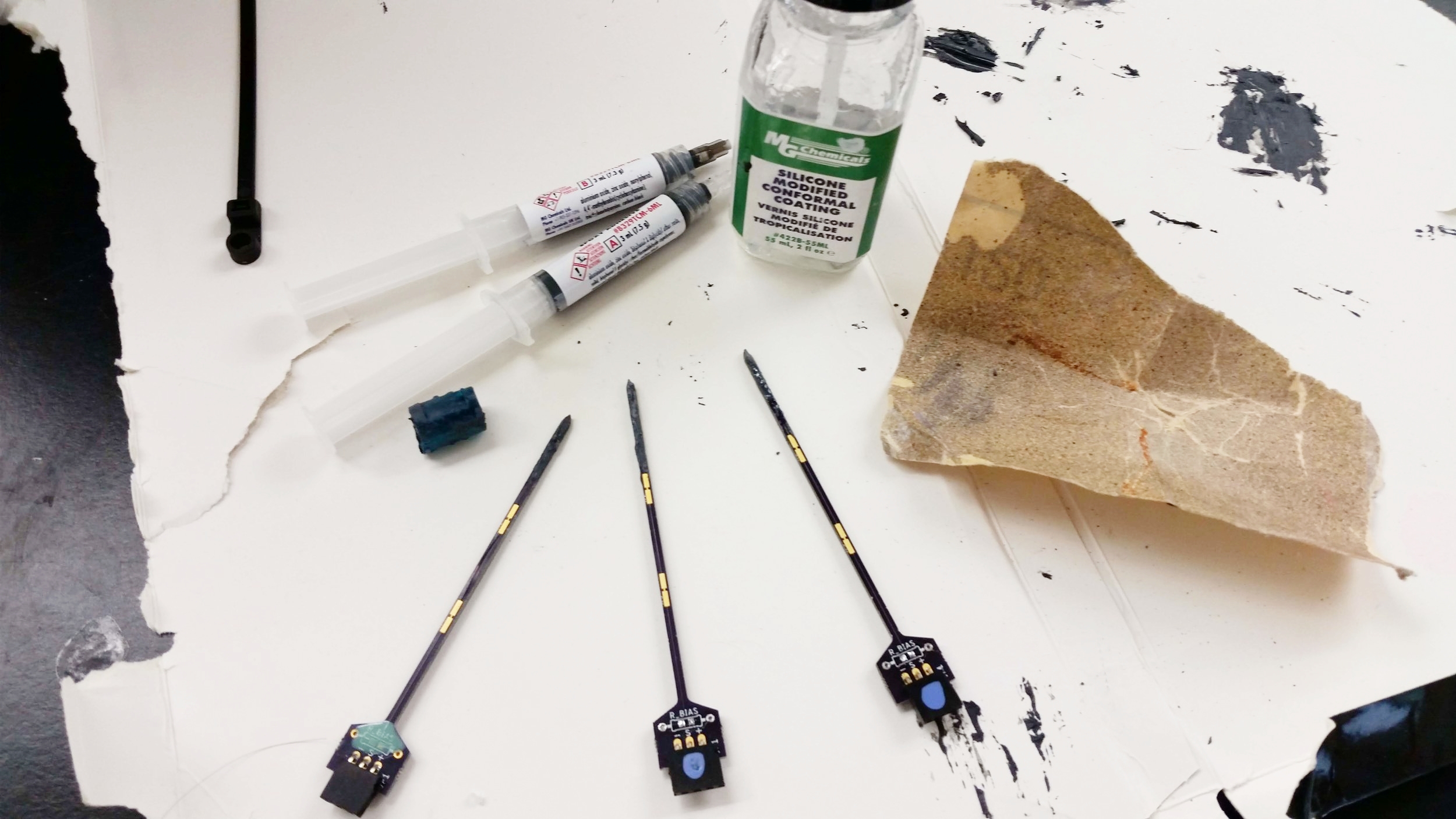
After the epoxy is set, gently wipe with sandpaper to remove any major impurities. Next, coat the entire probe with silicone conformal coating with two coats, letting dry completely in between. This will seal the epoxy to prevent plant moisture from seeping in and changing the properties of the probe over time. It will also waterproof the rest of the board. Make sure to avoid getting and silicone in the connector.
Step 4: Wire Things Up
The probes should be wired to the board as shown to work with the current code.
This wiring diagram does not include the SD card that is included in the code. It should be hooked up as per this tutorial with the chip select pin on the SD board going to pin 9 on the Feather and the SPI pins going to the corresponding pins on the Feather M0 (SCK, MISO, MOSI).
If you’re feeling savvy, feel free to play around with what pins are used. It’s important that the probes output goes to an analog in pin on the M0 (A0 to A5 shown below). The trigger can be moved to any pin, provided that the code is updated to match.
The heater probes could be attached to the 3.3V output pin (identified by “3V”) in order to further stabilize the power delivered as battery voltage decreases as it dies but the 3.3V should always be the same. However, this would reduce the energy efficiency of the system as the 3.3V output pin goes through the M0’s internal voltage regulator which burns off the excess voltage as heat. Also, the 3.3V supply has a max supply of 500mA which is near the current draw of a single heater probe.
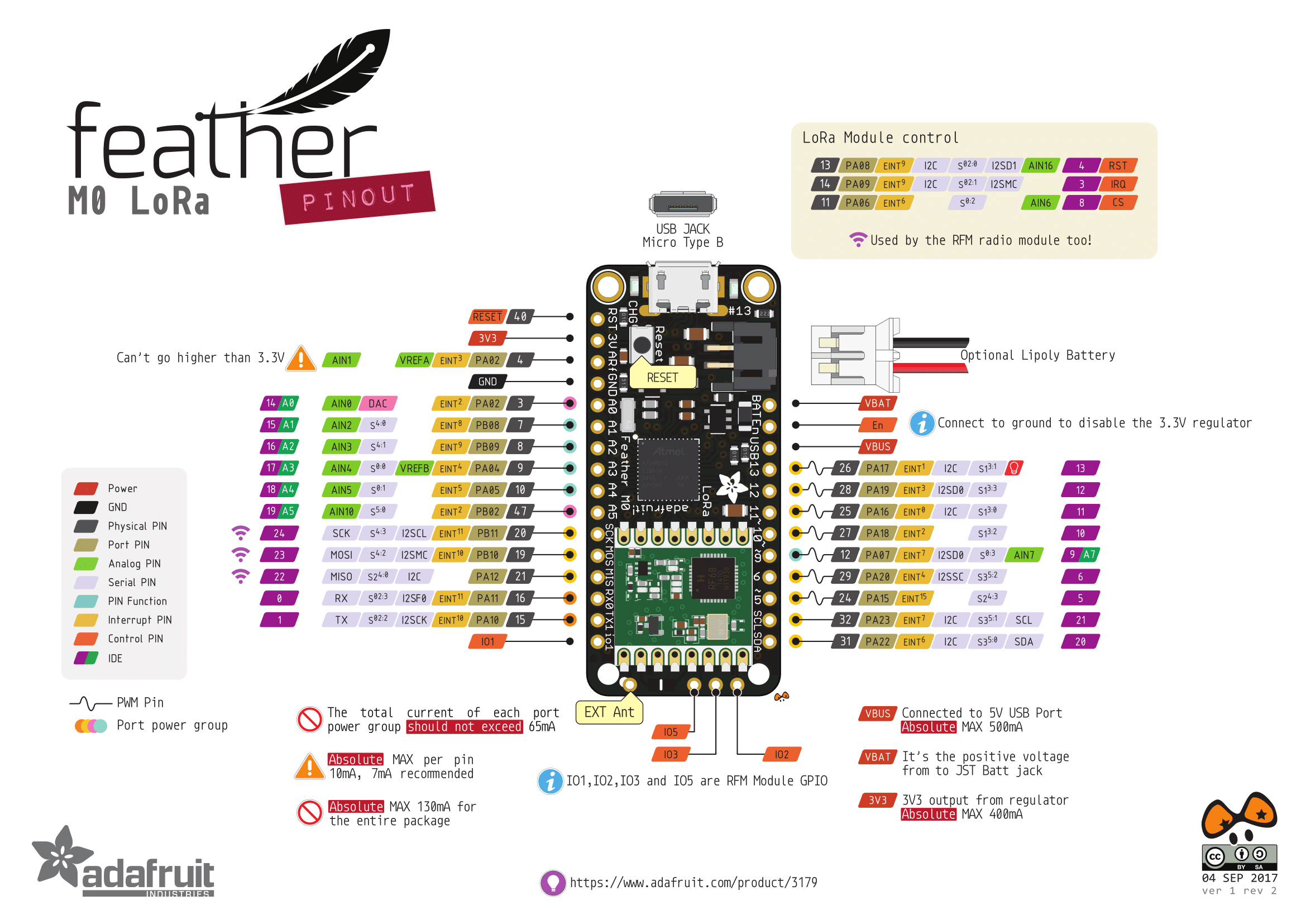
Pinout of Adafruit’s Feather M0 board. More information on the M0’s pins can be found on the Adafruit website at this link.
Step 5: Program the Microcontroller
The code for the basic program described in this build guide is posted at this link. A future blog post will walk through the important functions. Further in the future, a stand alone library and/or incorporation with project Loom is planned.
If you’ve never used an Feather M0 before, check out these two pages on Adafruit’s tutorial:
If you’ve never programmed in Arduino before (or ever), I would highly recommend reading though a few of the fundamental tutorial pages on the Arduino website until you grasp basic the basic concepts and idea of what Arduino is. Linked here.
Step 6: Install in Plant
This part of the process will change slightly based on what plant this is being installed into.
In order to to ensure that the probes are properly spaced, a 3D printed guide should be used. This version has a 7mm spacing between the probes. Future tests should test with different probe spacing. This doesn’t need to be as precise as the thermal epoxy mold; I used a Lulzbot Taz 5.
Insert the probes into their respective holes in the guide with the heater in the middle. Turn all of the PCB boards to face the thin side of the guide such that all the boards are parallel and facing to the same side (not up or down); this will help to deliver the heat pulse to the thermistors symmetrically. Optionally, use epoxy/superglue to fix them in place.
If you’re installing in a tree, holes will need to be drilled into the wood at a proper diameter (~2.75 mm) using an additional “guide”. As of now (6/11/2018) these have not been tested in a tree.
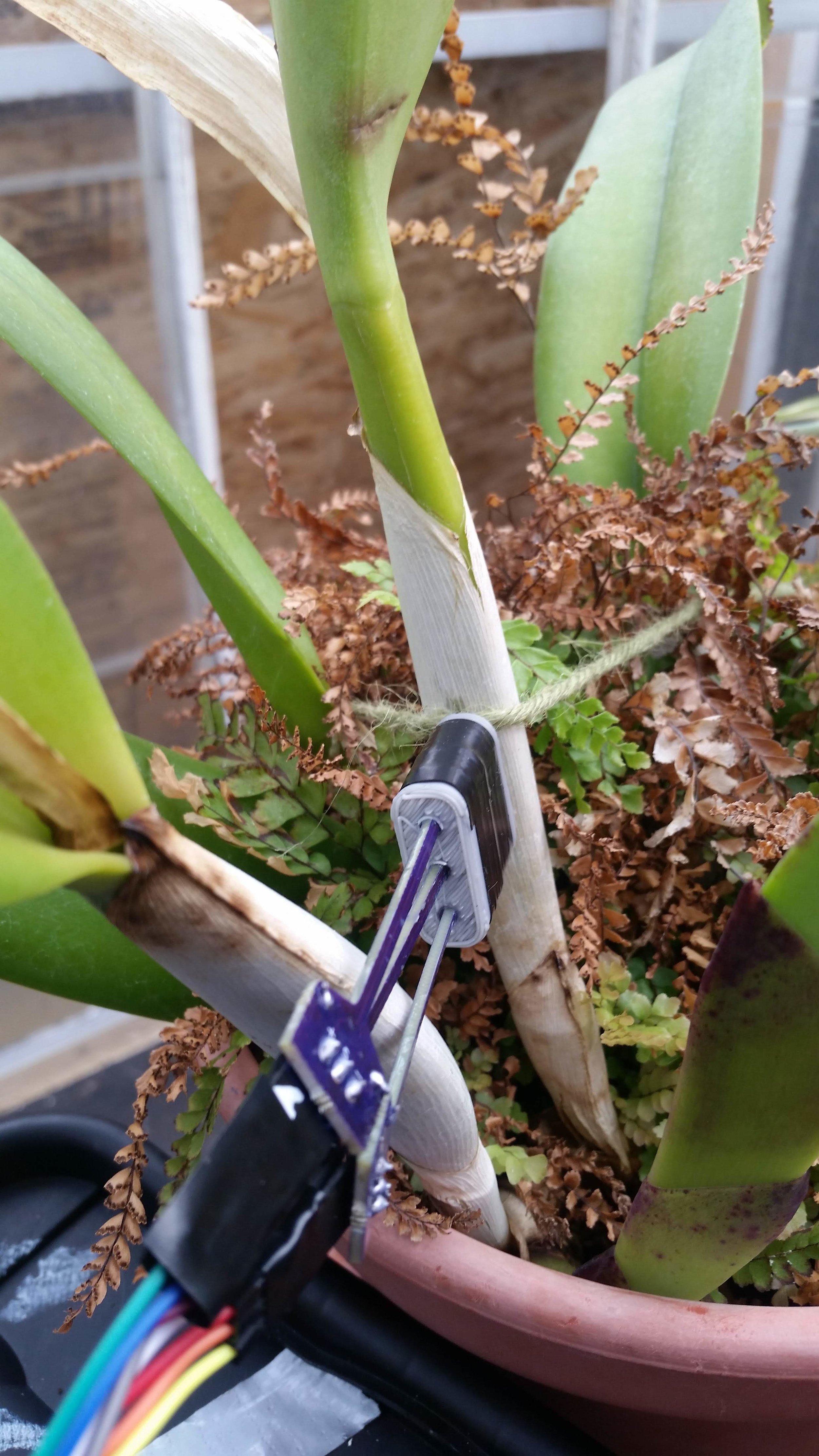
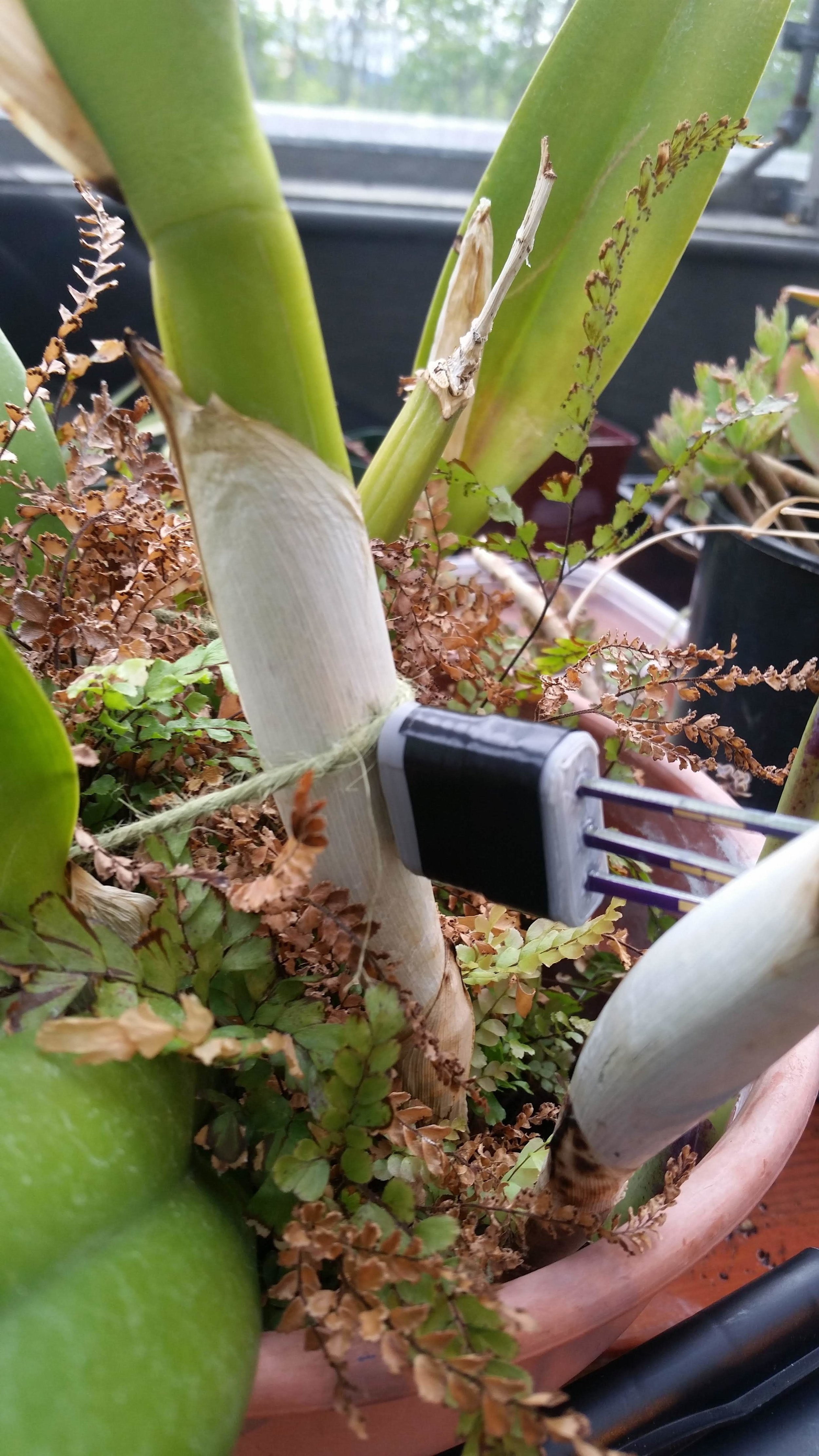
Probes installed in an Orchid. Notice the orientation of the probes, the pcbs are all facing the same direction.
Based on preliminary tests it should take about a day for the temperature to regulate and good data to start coming in. A later blog post will go into further detail on best practices for installing in different plants (especially trees) after some more tests are conducted. Potential things include: installing all probes in the north side of plants to avoid the sun (south if you’re on the wrong side of the world), filling any drill hole cavity with thermal grease via a syringe prior to inserting the probes (improve contact with the tree) and filling the end of the hold with putty/glue to seal it.
If you have any questions or suggestions for this design please please please reach out to me, Brett, at stoddabr@gmail.com. Happy building!
One metric for plant health is simply how “hydrated” the xylem is. This can be an indication of how much water the plant has been drinking and could change if it is living in a stressful environment.
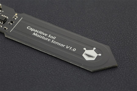
This sensor would be very similar to capacitance sensors used to measure volumetric water content (VWC) in the soil. An open sourced implementation of that is the Gravity Capacitance Soil Moisture Probe which is from DFRobot. It uses the TLC555I pulse generator to generate a signal which passes through a transmission line (on a pcb) that is immersed in the soil. Depending on the VWC of the water, the properties of that embedded transmission line changes.
Image of the Gravity SM Probe. Notice the transmission line going around the edge of the sensor. A thinner version could be implanted in a tree to determine “hydration”.
For the tree implementation, the transmission line would go along a probe similar to the one used for the thermal sap flow sensor.
By far the most annoying part of designing a thermal sap flux probe sensor is the “thermal” part. Without a proper heat pulse, there is no sensor. The problem is generating heat requires raw energy. According to my calculations, the heater makes up ~99% of the total energy requirements for this sensor. One of the goals of this project is to make the sap flow sensor as energy efficient as possible which will require a lot of testing to find the most efficient way to send out a heat pulse.
The Knobs
To find that maximum efficiency, there are a couple of design “knobs” that can be adjusted to find the maximum efficiency. Unfortunately, due to the short amount of time on this project, not all of these are going to be tested. Here is a list with what I believe are going to be the most important factors first:
Energy Delivered (joules)
Time of Pulse (second)
Depth into Tree (inches from the edge of the tree’s cambium)
There’s a possibility that a “wrap” sensor could be possible like Dynamax’s Dynagague which uses thermojunctions on a flexible PCB
Size of the Probe
The *IDEAL* Physics
I’ve put together a simple spreadsheet of a few different heater resistance values. Since this sensor is primarily being designed to integrate into other OPEnS Lab projects (namely the Evaporometer) a 3.7 voltage supply is assumed (uses 3.3V logic but runs off of a 3.7V battery, the heater will draw power from the battery).
One thing that should be noted when finalizing the resistance: the wattage rating for the resistor. There exists a lot of SMT resistors on the market, Digikey lists near 50 thousand, however, only a small minority possess the wattage requirements to provide that much heat (this can be seen in the “wattage” column of the attached table). If a resistor is chosen that does not satisfy the wattage requirements it will most likely fail. If a specific resistance is desired that is not available at this wattage, two identical resistors can be placed together in series, essentially halving this wattage requirement.
The temperature delta was calculated assuming that the heat capacitance of sapwood is 8 joules/C. This is an estimation.Further research into the exact heat capacitance of sapwood should be conducted.
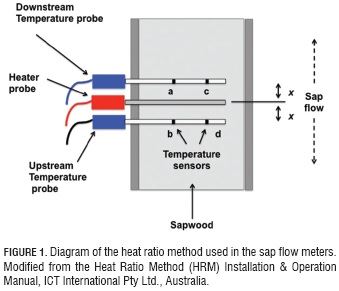
Thermal sap flux (or flow) sensors have been popular amongst environmental sensing experts since the mid-20th century. They measure the velocity of sap through the stem or trunk of a plant using an array of heaters and temperature sensors.
A modern sap flow variant, proposed by Grainer, is made up of two temperature sensing probes directly above and below a heater probe—all spaced evenly. When a measurement is taken, the heater probe turns on and emits a heat pulse for several seconds. Then the temperature difference between the upper and lower probe is recorded. The temperature difference over time can be used to track sap flow (the specifics of this will be talked about in a later blog post).
To construct a sap flux sensor using surface mount technology (SMT) which can be manufactured using an entirely automated setup given a pick-and-place machine but can still be made by hand by a person with adept soldering skills.
Challenges
The biggest challenge for this project is minimizing the width of the probes. Inserting any foreign object into the xylem of any plant will alter how sap flows through it. As such, minimizing the size of the probe is critical to accurate measurements. Current commercial probes have diameters of around 1.5mm (http://dynamax.com/products/transpiration-sap-flow/tdp-sap-velocity-thermal-dissipation-probe).
Limitations in commercial PCB etching process are a limiting factor in the minimum size of these probes. Also, if a sufficiently small probe size is achieved, the number of plant types this can be used on increases. For example, a large probe may only be used on trees of a sufficient diameter while a smaller one could be used on crops such as corn.
For the temperature sensor probe thermistors were chosen to be the sensor component. Thermistors were chosen because of their high level of sensitivity when compared to other sensors. Thermistors act as variable resistors that alter their resistance based on their temperature. The main drawback to using thermistors is that their output is not linear, but rather follows a logarithmic curve and so they are difficult to work with. For this probe, a voltage ladder was used to retrieve the resistance of the thermistor as shown in the schematic in the results section.
The heater element consists of a 50 ohm, US0603 footprint resistor with a 0.38 wattage rating. A future blog post will go more in-depth on how the resistance was calculated.
To maximize contact with the plant’s xylem, thermal epoxy was used in a mold around all three PCB probes. This was designed in SolidWorks 2017 and printed on a FormLabs Form 2 SLA printer for maximum resolution. The inside of this mold was coated in mold release spray to prevent the thermal epoxy from sticking to it. After the epoxy was sufficiently dried, a layer of silicone conformal coating was applied to waterproof each of the probes.
To control the sensor, a microcontroller with built-in ADC’s (here an Adafruit M0 Trinket) was used. The output pins on the temperature sensors were connected to the analog inputs of the microcontroller. An NPN transistor sat between a voltage source and the heater and was controlled by an output pin on the microcontroller.
Results
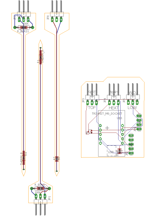
Images of the final PCB are shown below. It uses standard US0603 footprint resistors.
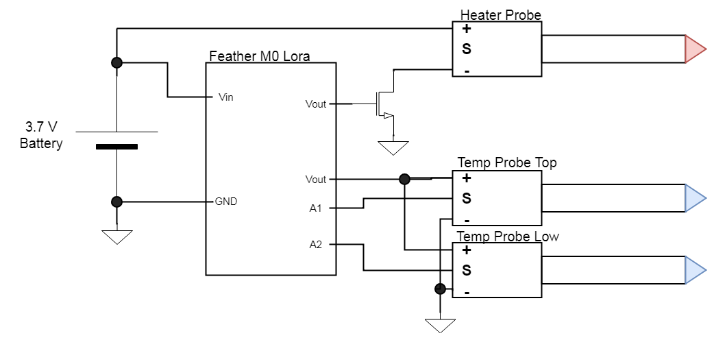
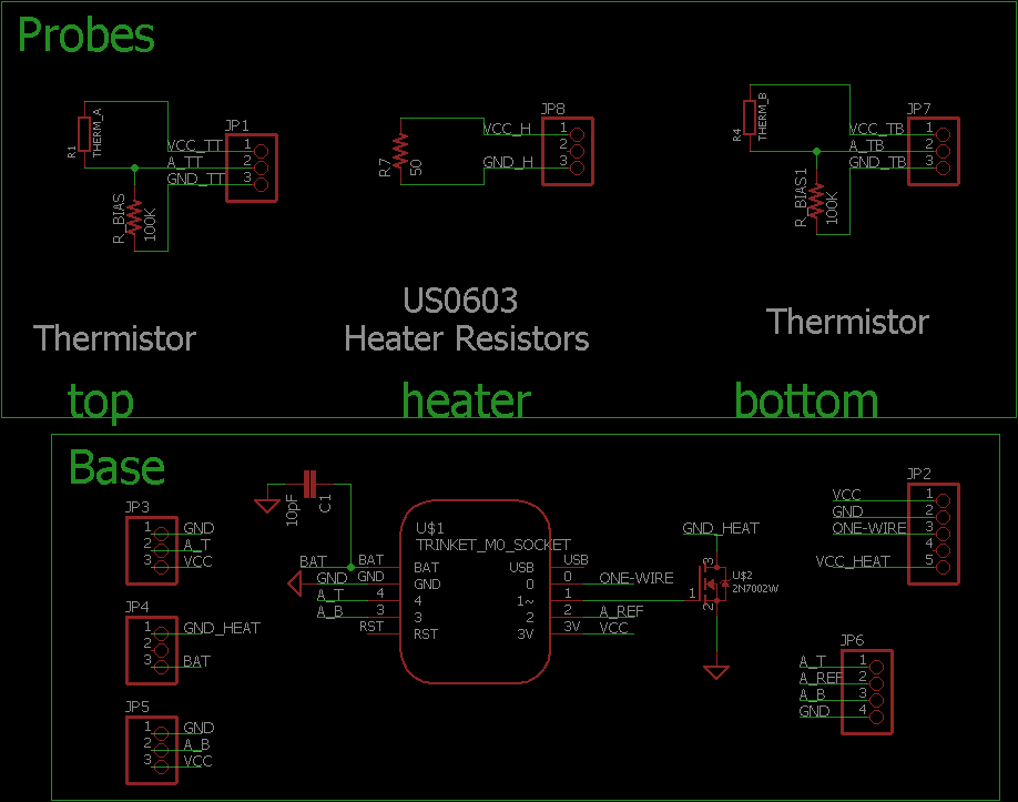
Schematic of the Sap Flow/Flux sensor with thermistor temperature sensors.
Image of the board design for Sap Flow sensor with thermistor temperature sensors. The two probes on the left are the thermistors and the one on the right is the heater probe. The PCB on the right houses an Adafruit M0 Trinket.
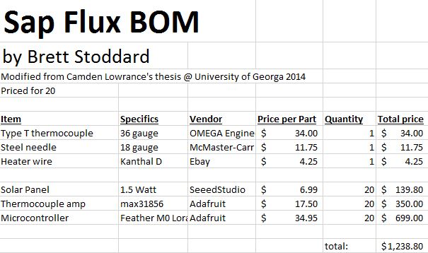
The bill of materials used is below.
A future blog post will go into a more detailed, step-by-step tutorial on how to build your own! It will also have finalized design files and best pracitces.
Room for Improvement
As with any project design, there are a multitude of ways that this could be improved. A few ideas with good potential are listed below in no particular order:
Linearizing voltage output using a parallel thermistor configuration
A/D conversion on the probe sensor to avoid signal loss across the line
Housing to protect the temperature probes from solar radiation
Insulation to protect the probes from ambient temperature fluxes
To test the probe described in my previous blog post, I deposited the probes in a banana plant I had handy.
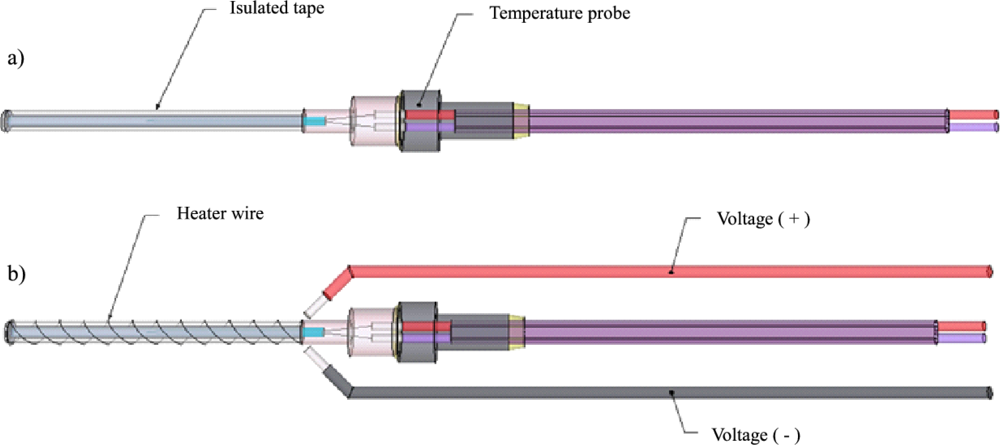
How I built the probes by inserting heater wire and type T thermocouples into hypodermic needles. More resources can be found in my last post and in the following paper by Davis et al. Post here. Paper here.
The graph result of the test is below:
As you can see, the top probe was not reading the correct temperature. This was probably an issue with the accuracy because it remained surprisingly precise meaning that the results shouldn’t be completely discarded. Daily trends are evidence that the sensor could be working somewhat. This is nowhere near the accuracy I intend to get with my final design.
However, there definitely is something interesting going on here. The data was recorded over an interval of three days. Examining the Differential plot, there seem to be roughly three major up-and-downs that PROBABLY are related to the day-night cycles of photosynthesis.
Before I got started designing the SMT sap flow, I built and tested the probe sap flow sensor popularized by Grainer. This design popular with researchers probably because of its inexpensive BOM ( ~$10/sensor ) and promisingly low labor ( 1 hour/sensor ) which puts the total price at ( ~$60/sensor ).
When I replicated several of these probes I found significant difficulty in making them. The 36 gauge wires are especially difficult to work with and the nichrome wire heater probe was almost impossible to wind to a high enough resistance. For the 7 I built, only 2 were usable enough to record meaningful data. This is not a process I would recommend to anyone.
The biggest difference is that I used a thermocouple amplifier chip instead of building my own. This greatly simplified the design and made fabrication a lot easier. I chose an Adafruit Universal Thermocouple Amplifier MAX31856 Breakout board. I made sure to set it to the Type-T setting. Adafruit has an excellent guide on how to use one of these on their website here.
The use of annealing ovens for 3D printed plastic is a useful technique that helps strengthen the plastic part and improves the overall look of the plastic. In this experiment, four 3D printed bag sealing caps were annealed with different techniques to compare the results. The annealing of ABS plastic is performed at a temperature range of 105C-107C which the glass transition phase of the plastic is. When ABS is printed, it is cooled below its glass transition phase which keeps the plastic harder and brittle. By slowly heating up the plastic to its glass transition phase the plastic begins to deform. This deformation is the breaking of the semi crystalline structure within the plastic to relieve stress that is created when the plastic is printed. When plastic is slowly heated, and this stress is relieved, the material is then cool very slowly so that the internal structure remains somewhat viscous- increasing overall strength of the material.
BACKGROUND:
The oven used to perform this experiment was a mechanical convection oven [Source]. The mechanically circulated air heats the plastic, and then melts it. The plastic parts are in the oven for the entire heating, baking, and cooling process. The error of the oven is estimated to be +-2C. [Source] Literature states that annealing can vary in process but most sources suggest the heating of the oven to the glass transition phase at a rate of 50F to 200F over the course of 2 hours. Holding in the oven 30 minutes for every ¼” of plastic (width) and then cooled 50F every hour. The purpose of the slow process is that the plastic is amorphous. Different parts of the plastic can be in different states at different times based on thickness and air exposure. In other words, there is uneven melting and cooling of plastics. The mechanical circulation of air and the slow process is supposed to account for much of these errors. If plastics are cooled or heated at different rates then different parts of the plastics can be in different states which could potentially weaken the part overall by creating stress concentrations; having a brittle location, a half-melted location, or a partially cooled location will disrupt the uniformity of the printed part.
EXPERIMENTAL:
Experiment one was conducted with a high range of temperature, revealing the importance of the glass transition phase temperature. The first cap was placed in the oven at a temperature of 50C and then slowly brought to a temperature of 108C over the course of 30 min. The 3D printed cap is ¼” in thick. After 30 min at this temperature, the cap was removed without cooling slowly. There was no difference in appearance or feel of the cap.
This cap was cooled for over 24 hours before being put back in the oven. The purpose of a second heating was to try and see a noticeable difference in the plastic. The second heating was conducted at a stable temperature of 121C. The total time in the oven was 1 hour 42 minutes. This much longer than the recommended time. When pulled from the oven, the caps were noticeably deformed with visible melting near the center. This warping was the plastic melting outwardly. This is not desired. The purpose of the glass transition phase is to melt the crystalline internal structure of the plastic without deforming the overall shape. It was concluded that the temperature was much too high and that the glass transition phase does hold precedence.
The next experiment tested an extended time in the oven. A cap was placed in the oven and the temperature was increased by 12-15C every 15 minutes until the oven reached 105-107C. The cap was then held in the oven for 57 minutes. After this, the cooling process began. The oven was decreased by 15-20 degrees every 15 minutes until the oven reach 50C. It was then turned off and allowed to cool to a temperature slightly above room temperature. This cap shrank slightly (3mm) which was noticed when the cap was not able to screw onto its respective bottle.
The above experiment was repeated, and it was found that this shrank as well.
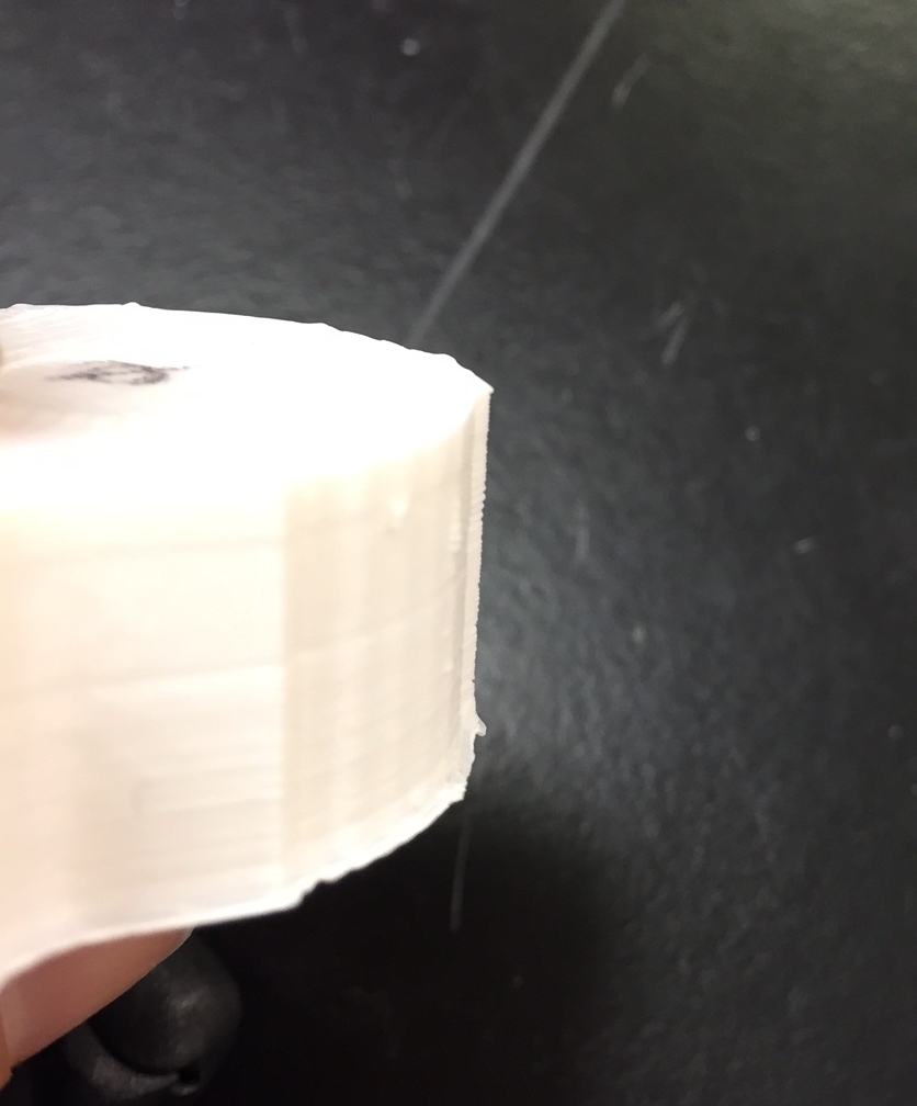
A final experiment was conducted with a newly printed cap. The oven was heated by increasing the temperature 12-15 degrees Celsius every 15 until it was brought to 105-107C (oven fluctuates slightly). The part was kept in the oven for almost 2 hours before the cooling process began. The oven was brought down to 50C in the same manner as above. The part was cooled to room temperature. This part also shrank by approximately 3 mm. The part, however, was also shinier than its un-annealed state, and was smoother after it was cooled.
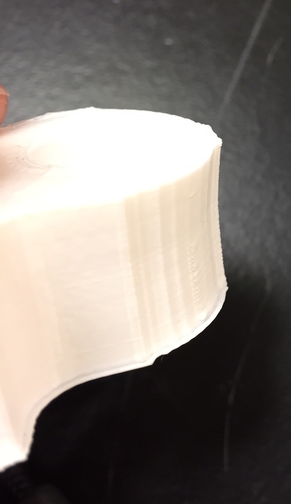
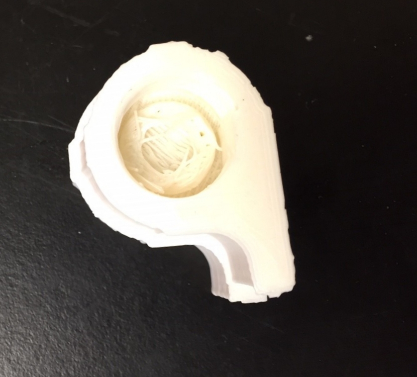
The pictures above highlight the difference between the annealed and the unannealed caps. The Annealed caps show the visual signs of warping and slight melting.
The photo above shows the shrinking that occurs when the 3D caps are annealed. There was little warping on this cap-temperature was correct- but shrinking still occurred which can be seen above with the unannealed cap is larger underneath the other cap.
CONCLUSION
Based on the above experiments, it could be concluded that annealing for smaller printed parts that need to fit counter parts (ie. Caps) may not be the most efficient method of finishing a part. The shrinkage of 3 mm could be accounted for in the 3D design process by adjusting dimensions of the design. There are, however, better methods that do not have such a large amount of shrinking involved. Also, if the goal of the annealing is for aesthetic purposes then vapor finishing is the suggested method. The unfinished cap has a diameter of 19 mm, a vapor finished one of 18 mm, and an annealed one of 16.5 mm. Future annealing experiments could be conducted on flatter parts whose max load tolerance could be measured- to test strength improvement-, or parts in which shrinking is easily accounted for. Based on the annealing of caps, however, the process was more cumbersome than necessary and vapor finishing with acetone is the recommended method for both these parts and parts similar in design. Vapor finishing accomplishes the same aesthetic results without the wait time and the shrinking.
Vapor finishing uses acetone to smooth finish 3D prints by filling the micropores present in the plastic that result from printing. The process of vapor finishing saturates the air around the part to make the surface “flow” into a smoother, better finish. There are two types of acetone bath; cold finishing and hot finishing, both use pure acetone to vapor finish the printed part. The benefits of cold baths being that the part can be left in the bath for multiple hours, and the fumes are more easily controlled. Boiling acetone (temperature of 132 degrees Fahrenheit) is a faster method than cold finishing. Results of boiling acetone can be seen in a matter of seconds, often outweighing the dangers of boiling the chemical [SOURCE]. By smoothing out a printed part the stress concentrations that are created when the part is printed, are decreased. This is done by decreasing the print lines and the micro-pores and micro-cracks in the plastic by essentially filling these in with acetone [SOURCE]. For both cool and hot vapor finishing, parts require a cooling time that ensures all the acetone has been evaporated and that the part has completely hardened. To make sure of this, pieces could use 12-18 hours before being implemented in designs. This will also make sure no warping or pooling of the acetone has occurred between ridges on the part.
DESIGN:
The vapor finishing design for this experiment included a rice cooker chamber, acetone, 3D printed parts, and scale. This is the easiest method of boiling acetone. For each 3D cap, the time left in the bath, the temperature, and the time allowed to cool was kept constant. The part was placed in the chamber, the specific amount of acetone was added, and then the heat was turned. The heat was kept on for the same time for each bath, before being turned off and the lid to the chamber was removed. The part was then massed and used. For each experiment, the heat was turned on for 45 seconds to allow the acetone to completely vaporize. The lid was then removed when one minute had passed. Each part cooled for 15 minutes before being tested. The cooling period was implemented to make sure that excess acetone was evaporated, and the part was hardened.
Summary of Test one:
A total of 10 trials were conducted with acetone levels ranging from 0mL to 19.1mL of acetone. It was found that when a cap was treated with 0mL of acetone there was a percent mass gain of 31.3% while a cap treated with 19mL has a percent mass gain of 16.6%. Mass gain was measured by weighing the caps prior to finishing, letting them cool after finishing, and then screwing them on a bag and squeezing the bag while it is upside down. This meant water was absorbed into the micropores when water was forced into the plastic. Caps in between these two points included 5.3mL with a mass gain of 31%, 10.8mL with mass gain of 19.7%, 14.1mL with mass gain of 21.4%, 16.3 mL with mass gain of 18.5%, and 17.8 mL with mass gain of 18.5%. The other trials were repetitions of these levels with similar results. Other data take in experiment one was the water lost from the bag when the caps were being tested. The initial amount of water was measured in mL. After the bag was tilted and squeezed, the bag was re-massed to see how much water escaped. It was discovered that the more acetone used, the less water that escaped. The untreated cap allowed almost all the water to escape. The cap treated with 19mL only allowed 1.7mL to escape out of 140mL.
Summary of Experiment 2:
This experiment was performed to confirm the results from experiment one. The focus was on one low level acetone level and then many higher-level acetone levels. Since the first experiment established the necessity of the higher levels of acetone, the second experiment was performed to finalize this conclusion. For comparison, an untreated cap was tested with the bag and, again, it allowed lots of water to escape with some pressure, further supporting the need for vapor finishing. Experiment two did support the first one. An additional five trials were completed. One with no treated and four more, all above 17mL. The average mass gain between these four treated caps was 22.7%. These four caps allowed virtually no water to escape when attached to a bag and squeezed upside down, further supporting the conclusion made from experiment one. The untreated cap allowed almost all the water to escape again. The recommended amount of acetone was concluded to be 14-19mL.
Miscellaneous:
Weight of dry cap average: 5.18 g
Weight of cup used to measure acetone: 19.2g
Mass of bag: 11.4 g
Time to dry for each trial: 15 minutes
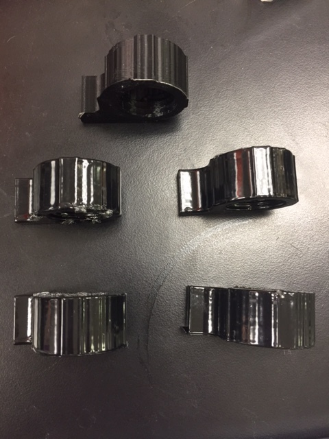
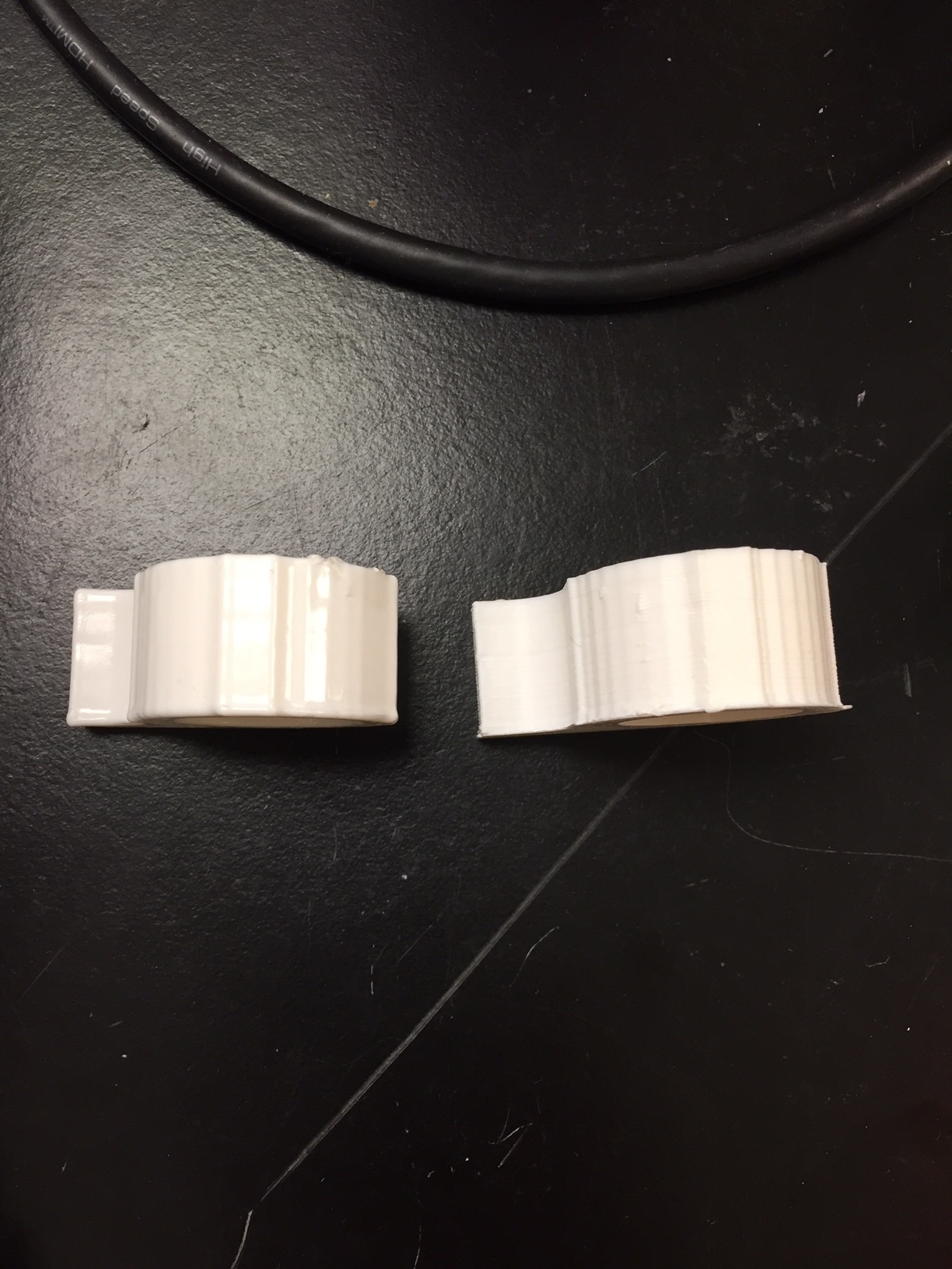
The photo above compares and untreated cap (top) with the treated caps. There are few noticeable differences, besides the greater amount of rounding in the 19mL level cap (top left).
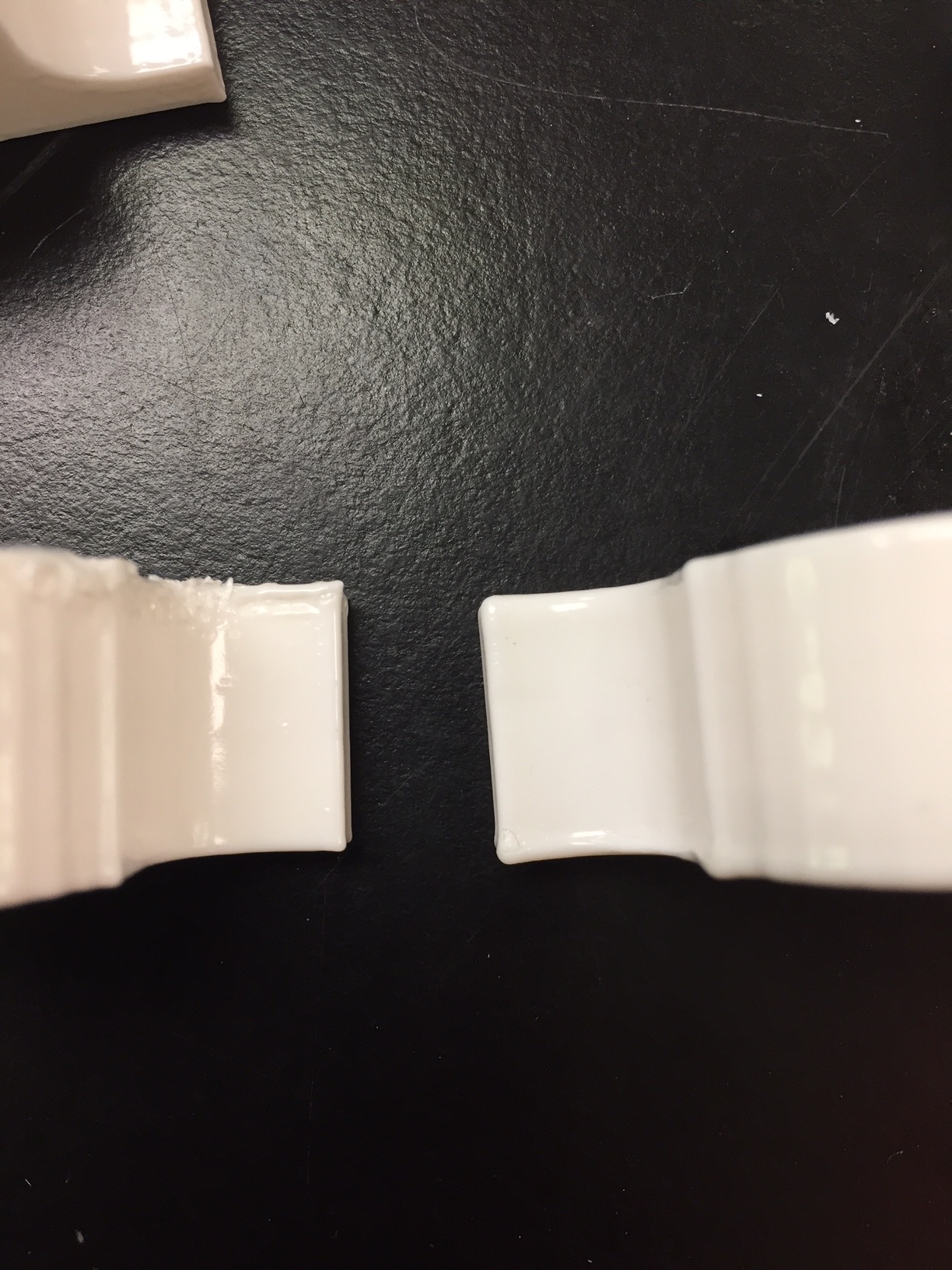
The above picture shows a cap treated with 10mL (L) and a 19 mL (R). The 10mL treated cap is less smooth than the 19mL treated cap. The edges are less rounded. The necessity of more acetone was also supported when the 19mL treated cap allowed less water to both escape the bag and cap connection and infiltrate the cap.
The picture above shows a cap finished with 19mL of acetone (L) and an unfinished cap (R).
The treated cap is much shinier and smoother than the untreated. There are decreased print lines and the texture is more uniform than the untreated.
CONCLUSION
Without any vapor finish, cap and bag connection allowed water to easily escape from the connection point with basic pressure. The largest increase of mass was also associated to the cap without any vapor finish, indicating that water was easily infiltrating the plastic. For the second experiment, the untreated cap did not have a large mass increase, but still allowed water to run out easily.
Increasing the amount of acetone used decreased the amount of water allowed to escape while also increasing the efficiency of the connection. Almost no water escaped at the connection point with even greater pressure compared the pressure applied to the little to no acetone experiments. This was also demonstrated simply by allowing the bag to tilt upside down and seeing that the parts treated with more acetone had less water escaping than untreated parts. The recommended range for small to medium parts is 15-18 mL of acetone. With that in mind, it was also found that levels of 19mL and 17mL both performed well under applied pressure but the 17mL acetone levels kept the exactness of the design better. Meaning the acetone did not smooth the part on the outside as much but performed just as well, and the differences were not very noticeable.
The mass of the caps was measured before and after each trial. To give an idea of how much water was being absorbed during each trial. For each cap treated, when attached to the bag, pressure was applied to test how this affects the amount of water escaping at the bag and cap connection. After pressure was applied and water was allowed run out. It was found that past 17 ml of acetone far less water escaped at the connection. The percent mass gained by the caps at this point was also less. This indicates that the increase in acetone levels helps decrease the amount of water soaking into the part. The greater the acetone levels, the better the webbing formed between the plastic layers. Increasing the acetone that is vaporized increases the acetone that is being deposited between particles in the plastic. This is also why a drying period is necessary to make sure the part has hardened sufficiently before use.
The amount water present after the bag has been squeezed was measured as well. This accounted for any water that escaped the cap through the pores during this process. It was observed that even though the caps still absorbed water with later runs, it was a small amount and most of the water leaking out was at the connection point. This was not performed for experiment two since experiment two was conducted to support the conclusion of experiment one.
Possible errors for this experiment were the acetone bath which could account for the increase in mass for many of the caps. Even though the finished prints were allowed 15 minutes to dry, that could not have been long enough to account for the acetone saturation. To ensure that the acetone is completely dry, the prints were re-massed and retested after more than 24 hours had passed. It was found that after these 24 hours, the difference in masses for the caps was no different. The top of the cap was less malleable after all the acetone could dry. For future printing, it is encouraged to allow the finished part to dry for a least a couple of hours to make sure all acetone has evaporated.
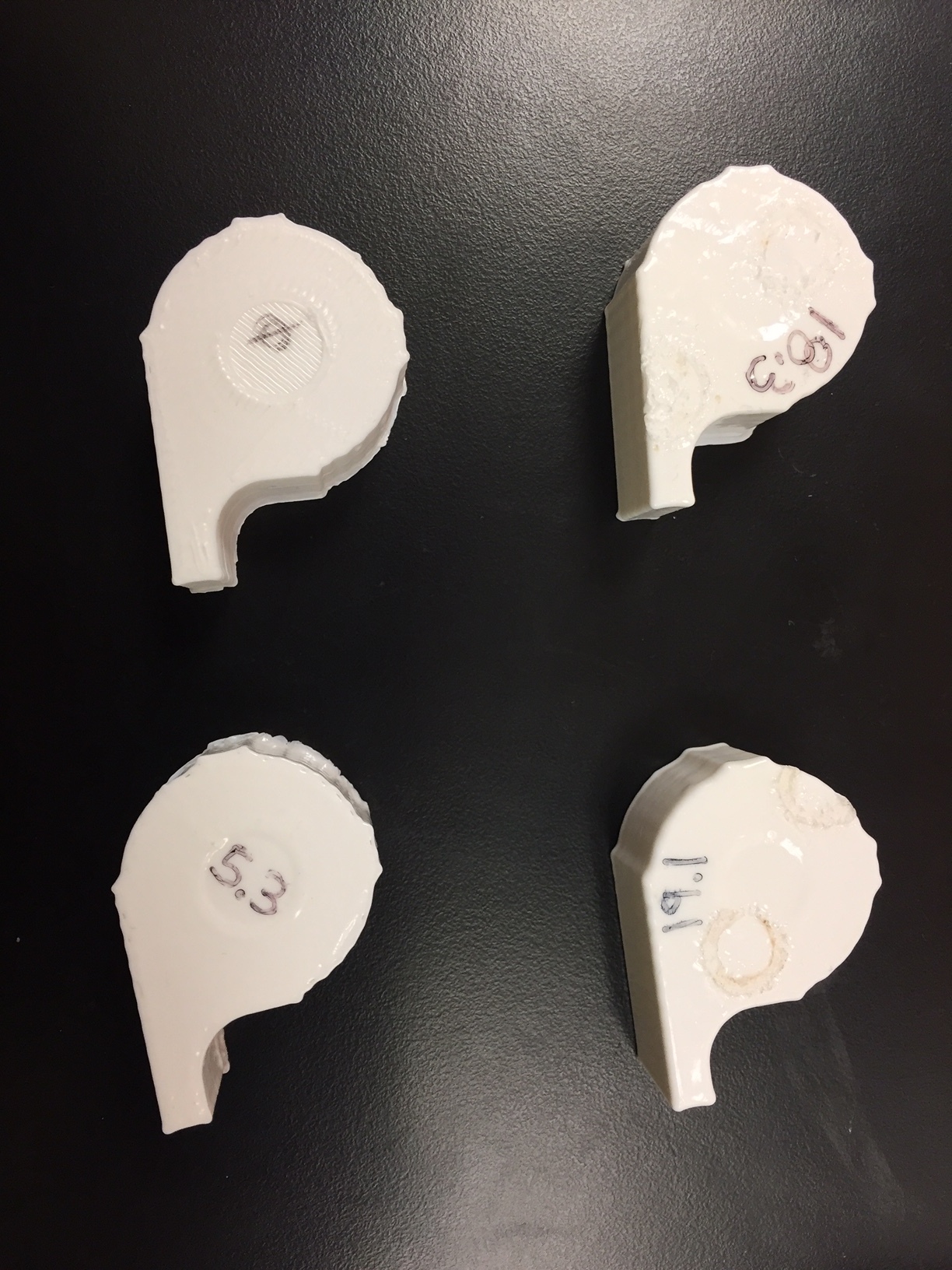
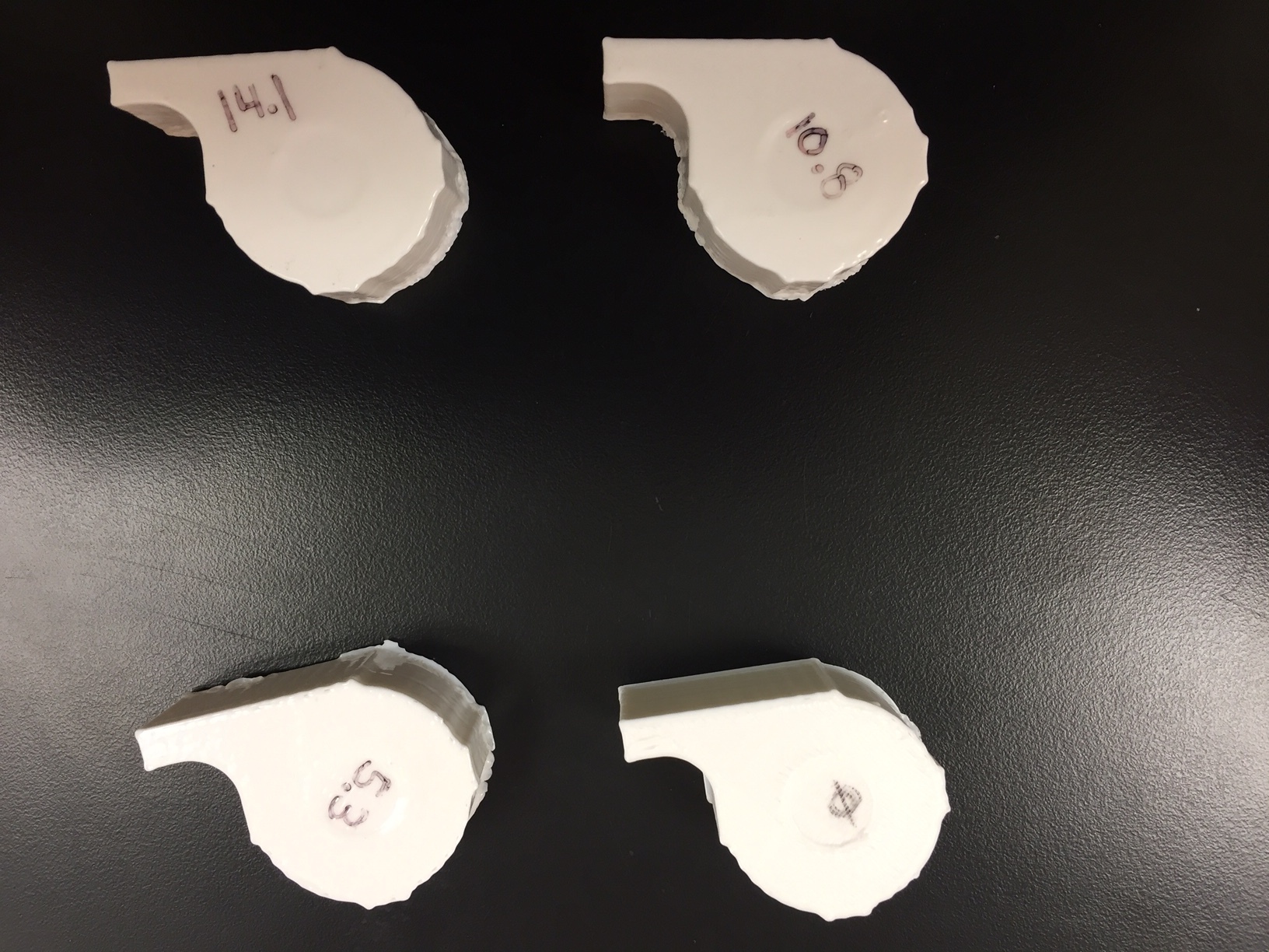
Below are pictures that compare the results of different levels of acetone. This can be used a reference to show how increasing the amount, increased the layer of acetone that finished the part. The results on the outside show increasing smoothness and rounding at the edges. Internally, increasing the acetone resulted in a better seal. There was not a great difference between the 18 and 19 mL caps, which is why the interval of 14-19mL is the recommended interval for the acetone. The numbers on the cap indicate the amount of acetone used in the experiment.