Author: Chet Udell
1. Introduction
The spatial and temporal distributions of CO2 at the earth-atmosphere interface and at the boundary layer above it are of great importance for soil, agricultural and atmospheric changes. In general, the source of elevated CO2 concentrations at this boundary layer depends upon root respiration and soil microbial activity (Blagodatsky and Smith, 2012; Buchner et al., 2008; Nakadai et al., 2002).
Improvement of CO2 gas concentration detection could lead to a better understanding of the agricultural cycle and the transport mechanisms at this critical interface. Moreover, better monitoring methods to detect CO2 concentrations can provide improved modeling and decision-making to enhance agricultural productivity. Until recent years, the techniques for detecting CO2 concentrations included only stationary sensors that give close-range readings or the use of remote sensing platforms, which have limited accessibility due to their high costs and relatively low resolution (Toth and Jóźków, 2016). In addition, the use of remote gas sensing is usually inapplicable inside greenhouses.
The growing use of open open-source hardware (e.g., Arduino) for research purposes creates new opportunities to bridge the gap between CO2 detection at high resolution and affordability. In agriculture, the use of open-source hardware and sensors for CO2 gas sensing is still novel with little supporting research. However, recent research has revealed the possible applications of operating such gas sensing systems for agricultural purposes. For example, the use of an open-source gas sensing device to detect CO2 concentrations in a rectangular greenhouse (106 m × 47 m) was recently proven by Roldán et al. (2015). Using a low-cost electrochemical CO2 sensor, they provided a high-resolution CO2 concentration map inside a greenhouse. Their device also had temperature, relative humidity (RH) and luminosity sensors. All of the data from these sensors can be used for better greenhouse operation decision-making..
The aim of our research is to evaluate CO2 concentrations and dynamics using new CO2 (NDIR technology) and O2 (UV technology) sensors inside a greenhouse. We aim to integrate these gas sensors, together with temperature, RH, and luminosity sensors, on a single logging device to gain high spatial and temporal resolution of the greenhouse environment. In addition, we aim to make the device small and transportable to eventually deploy it on a drone or a rail system to get location-tagged data throughout the greenhouse.
2. Materials and Methods
The sensors used in this project are detailed on Table. 1. All sensors were chosen according the following guidelines:
(1) Sensor accuracy similar to that of a laboratory sensor. For example, the CO2 sensor should have the same accuracy range as other CO2 sensors that were reported in recent published studies.
(2) Only off-the-self, open source sensors.
(3) The sensor should be low-cost compared to other existing sensors.
(4) Only sensors that are modular and light-weight, such that the complete system will be light-weight.
Table 1. Details of the device sensors. The “Name/Model” column includes links for each sensor’s web site. Total cost of sensors (without the optional GPS Logger Shield) was less than 300 $.
[ coming soon ]
3. Results and discussion
System integration included all the sensors detailed in Table. 1. Picture of the device and connection scheme are detailed in Fig. 1-A and B, respectively. Two power connections were tested: a 9V battery and a fix connection to wall power using a 9V adapter. The advantage of using the 9V battery is the mobility of the device; however it was sufficient only for ~5 hr when logging data at 5-min intervals.
 Fig. 1. Device description, (A) a photo of the device in the laboratory, (B) connection scheme of the different sensors.
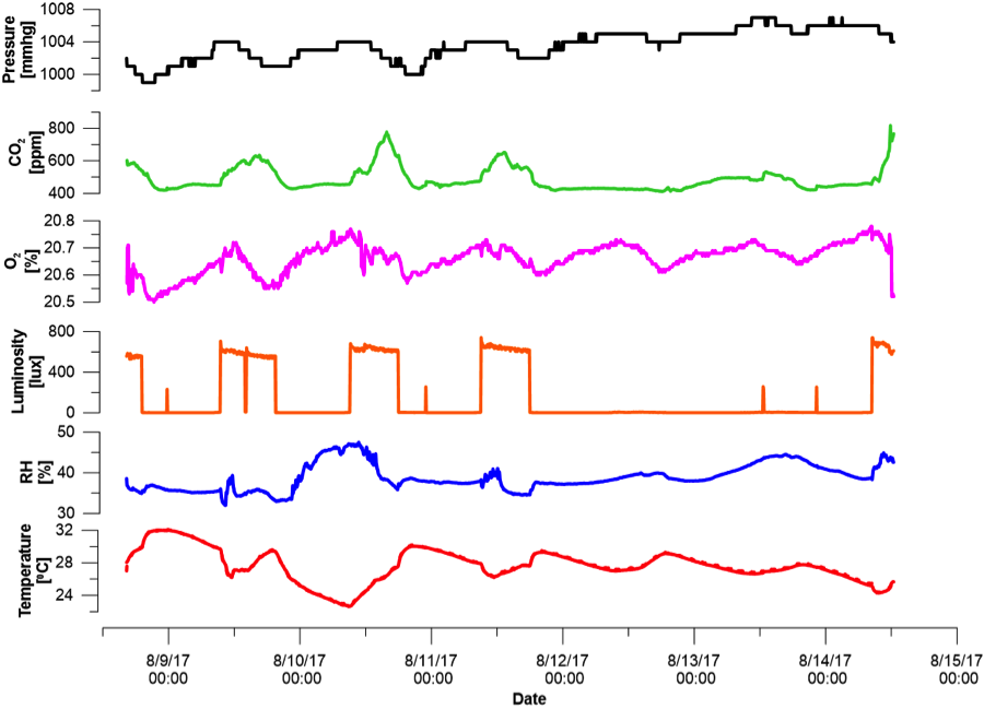 Fig. 2. Time series results from six days in the laboratory.
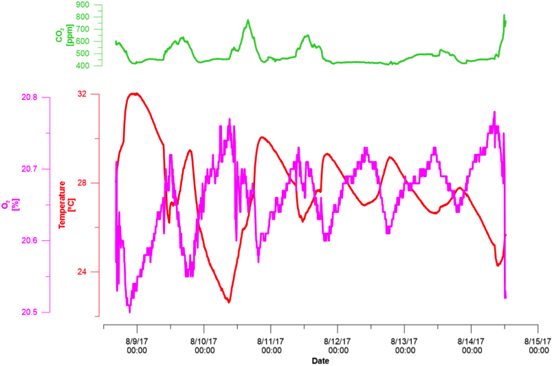 Fig. 3. Temperature effect on the O2 measurements.
Second deployment of the device was in an agricultural greenhouse located in Oregon State University, Corvallis, Oregon. The device was installed in the end of the greenhouse; ~5 m from the window and ventilation entrance (Fig. 4-B). To achieve reliable measurements, direct sunlight on the sensors was blocked using a cover installed 4 cm above the device. The cover was only above the device, such that air could freely circulate between the device and the surrounding greenhouse air. The only sensor that was exposed to direct sunlight was the luminosity sensor. Taking measurements in the shade is considered as standard procedure (for more details, see the “American geoscience institute” website). Moreover, shade is essential for the CO2 sensor because this sensor uses infra-red technology (radiated heat energy); thus exposing it to direct sunlight will bias the measurements by changing the infra-red energy in the sensor.
Results from the greenhouse measurements are shown in Fig. 4-A. Temperature and RH had the same typical daily cycles as shown in the laboratory data. During daytime, air temperatures were higher with lower RH values compared to nighttime. We note that the Y-axis scales are different between the greenhouse and the laboratory because of higher diurnal cycles in the greenhouse (no AC was used). Luminosity sensor reached full saturation (40,000 lux) during daytime, which indicated direct sunlight inside the greenhouse. Two reasons can explain the “noisy” luminosity readings shown in Fig. 4-A. First, the presence of clouds that temporarily decreased the light entering the greenhouse, and second, the fact that the device was measuring only at a single point below the plant leaves, thus the reading were subject to shade influence according to the angle between the sun and the leaves above the device. CO2 had a small diurnal changes in the scale of a few tens of ppm. These oscillations were within the sensor accuracy limit (± 30 ppm ± 3 % of measured values), and therefore cannot be observed using this sensor model. We note that the experimental greenhouse that was tested here was only with a low density of plants (i.e., number of plants per greenhouse area). In high-dense greenhouses, such as commercial tomato greenhouses, the overall photosynthesis will be much greater, causing CO2 daily oscillations above 100 ppm and thus the CO2 sensor will be more relevant. O2 dependency on temperature was the same as in the case of the laboratory measurements and not because of actual changes of the O2 in the greenhouse air.
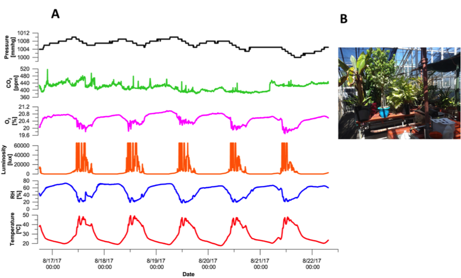 Fig. 4. (A) Time series results from five days in the greenhouse, (B) a picture of the greenhouse taken from the entrance door.
We also tested the use of a GPS Logger Shield to get position readings inside the greenhouse. In this case, the shield replaced the real time clock and the microSD board. The accuracy of the GPS position is highly dependent on the greenhouse roof material. In our case, the position readings were not stable with maximum offset of 32 m compared to the true device position inside the greenhouse. Results of the GPS readings are shown in Fig. 5-A were each re point is a single position reading and the green point is the true device position. The number of satellites for each reading is shown in Fig. 5-B.
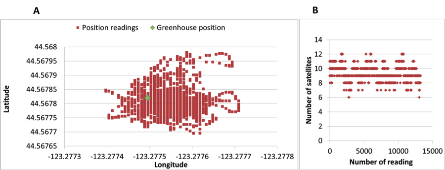 Fig. 5. GPS experiment, (A) GPS positing readings from one fix position inside the greenhouse (green symbol marks the true position), (B) number of satellites in each reading.
4. Summary
Integration of the different device sensors was successful and two 5-days measurement periods were conducted inside a laboratory and a greenhouse. Main conclusions at this stage are: (1) temperature, RH, and luminosity sensors were reliable and in the desired accuracy range, (2) problematic dependency of O2 sensor with temperature, (3) CO2 accuracy was not sufficient to measure the daily CO2 oscillations inside the experimental greenhouse.
We are now focusing to achieve the following objectives until the end of 2017: (1) improving the code for better power consumption; (2) validation of our CO2 sensor against a standard laboratory CO2 sensor that is frequently used in academic studies – IRGAs GMD-20 manufacture by Vaisala; (3) deploying the system on a drone or on a HyperRail device to obtain spatial greenhouse data and not only fix point measurements. The HyperRail is a low-cost rail system originally designed for moving a hyperspectral camera inside a greenhouse (additional information can be found in this link); (4) finalizing a short paper on the integration and deployment of the system in a greenhouse, which is now in preparation.
5. References
Blagodatsky, S., Smith, P., 2012. Soil physics meets soil biology: Towards better mechanistic prediction of greenhouse gas emissions from soil. Soil Biol. Biochem. 47, 78–92. doi:10.1016/j.soilbio.2011.12.015
Buchner, J.S., Šimůnek, J., Lee, J., Rolston, D.E., Hopmans, J.W., King, A.P., Six, J., 2008. Evaluation of CO2 fluxes from an agricultural field using a process-based numerical model. J. Hydrol. 361, 131–143. doi:10.1016/j.jhydrol.2008.07.035
Nakadai, T., Yokozawa, M., Ikeda, H., Koizumi, H., 2002. Diurnal changes of carbon dioxide flux from bare soil in agricultural field in Japan. Appl. Soil Ecol. 19, 161–171. doi:10.1016/S0929-1393(01)00180-9
Roldán, J., Joossen, G., Sanz, D., del Cerro, J., Barrientos, A., 2015. Mini-UAV Based Sensory System for Measuring Environmental Variables in Greenhouses. Sensors 15, 3334–3350. doi:10.3390/s150203334
Toth, C., Jóźków, G., 2016. Remote sensing platforms and sensors: A survey. ISPRS J. Photogramm. Remote Sens. 115, 22–36. doi:10.1016/j.isprsjprs.2015.10.004
VAISALA, 2012. How to Measure Carbon Dioxide [WWW Document].