The last post was about getting the HyperRail working with basic code. I have now improved the coding to give the user more control. The user can now control RPM and I have added some other functions.
Objective:
I intend to give an update on the programming of the HyperRail and new features the new code has.
Materials and Methods:
All was done using the Arduino IDE and all the code used for in this iteration can be found here.
There are currently two pumps to choose from for the OPEnSampler: a low flow rate, unknown-precision peristaltic pump and a high flow rate, “low precision” pump. They have their pros and cons and this writeup will discuss the angles of attack for deciding which one is more appropriate for our system.
Specs:
The WMC Pump has the following specs:
12V DC 400mA
297 mL/min flow rate, among other lower flow rate options
5mm Viton Tubing, among other options
Barbed Fittings
The Honlite Pump has the following specs:
12V DC 1.2A – 3.2A
1100 +- 8% mL/min flow rate
Tygon Tubing, among other options
Compression fittings for 1/4” OD tubing, among other options
Discussion
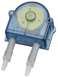
WMC Pump Head
The WMC pump has been tested on our prototype system and has proven to be reliable and true to its specs. It can reliably pump 250mL/min of water at zero net suction head, which is about three times as fast as our previous dual-pump system. Despite such an improvement, the flow rate is still quite low for attaining representative samples of suspended sediments, such as fine-grain sands [source]. A flow rate of 530+ mL/min is required to reach the EPA’s recommended 60 cm/s minimum line velocity for such sampling where the flow of the analyte heavily relies on the mass and specific gravity of the particulates [source].
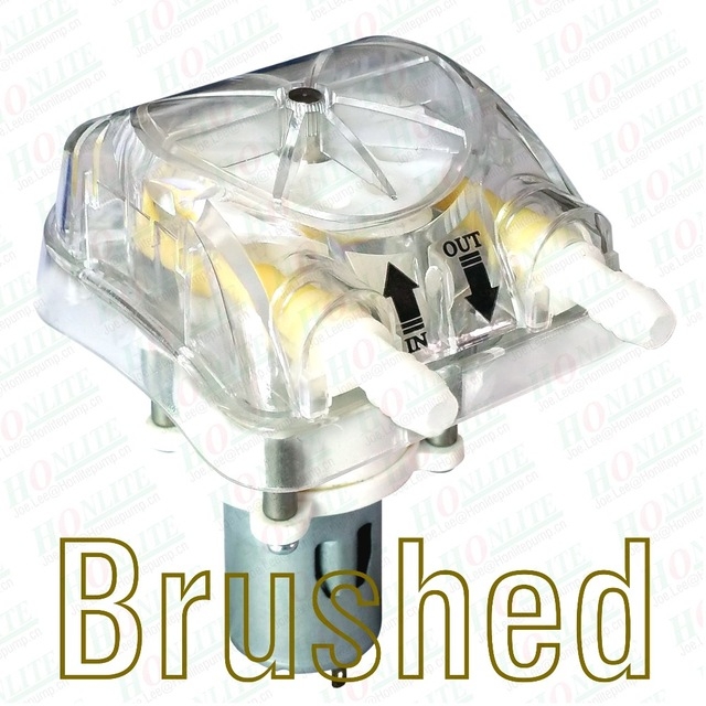
Honlite Peristaltic Pump
The Honlite pump from AliExpress has yet to be tested however the manufacturer supplies more specifications than the WMC pump. The defining characteristic of this pump is its 1100 mL/min flow rate at 12VDC, almost 4 times the rated flow rate of the WMC pump and twice the minimum recommended flow rate for sampling suspended solids. Some downsides are its high variance in flow rate of 8%, though further testing of the WMC pump could prove this is not an usual variance, and further testing of the Honlite pump could prove this variance is controllable. The pump head only has two rollers (three is standard) and so the rhythm of the pump could be noticeable, but will quite likely have a negligible effect on the sample quality.
One method of fixing the inconsistency of any pump used is to add a flow rate meter in series with the pump line. This flow rate meter can catch when the pump is struggling or increases its velocity significantly and adjust the PWM control of the pump driver chip, effectively increasing or decreasing the voltage supplied across the pump to account for the change in flow.
Conclusion:
Both pumps cost around $65 (the Honlite pump costs $30 with $35 shipping to the US) so reliability and flow rate are the most significant factors. Neither pump states its maximum suction head, though almost all peristaltic pumps seem to have a maximum suction head greater than 5m. This is why the Honlite pump was chosen for the Q4 2017 design, but several WMC pumps will be purchased as backups in the event we find the Honlite product to be faulty.
It is quite difficult to find a peristaltic pump with a sufficient flow rate for such a low cost and this is the primary source of skepticism for using the Honlite pump. How are they able to achieve such a large flow rate without increasing cost? The answer could be they are mass producing these pumps in a highly efficient system, or perhaps their pumps are not as reliable. Consistency in sample volume may not be a large concern, however an inconsistent sample volume is almost exclusively caused by a varying velocity of sampled water in the tubes. This varying velocity can certainly lead to varying turbidity and suspended solids measurements [source][source], and so consistency is a huge factor in choosing a pump.
An RGB light sensor we evaluated for use in the Evaporometer project. This sensor measures RGB, color temperature, lumens, and visible light spectrum, and has features that currently aren’t useful for our project, but are still worth documenting in this post.
Setting up the sensor:
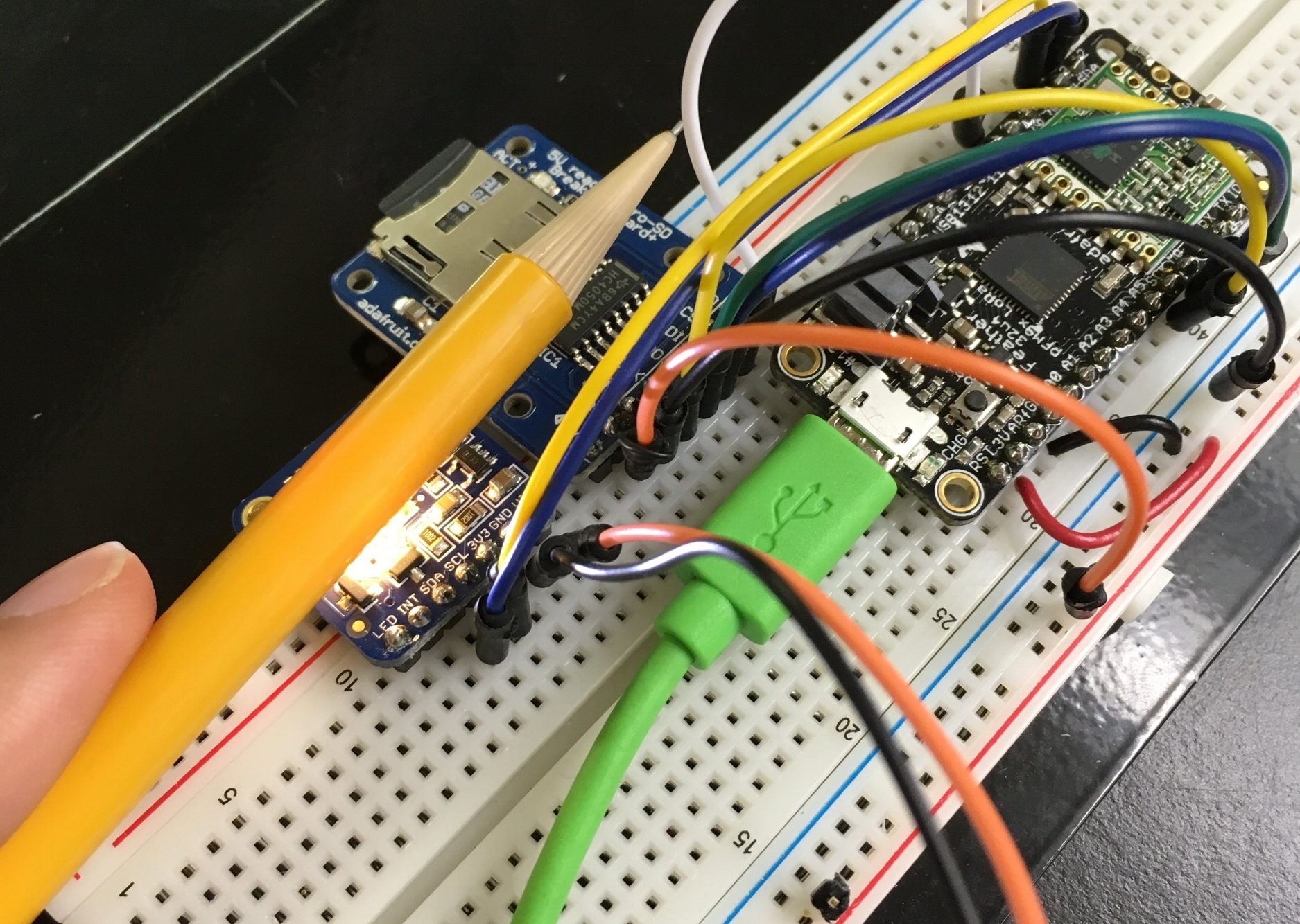
The TCS34725 was connected to an Adafruit Feather 32u4 using traditional I2C, although the RGB breakout features an additional port for a RGB LED to mimic the RGB values read by the sensor. More on the full functionality can be found on Adafruit’s website here. An SD card breakout was also connected to store the RGB, color temperature, lumens and visible light spectrum values.
A sensor right next to the white LED reads the RGB values of light reflected by different objects.
Testing the sensor:
For this test we were most concerned with measuring RGB values. Color could be read by reading the different colored light that was reflected by an object. A built in white LED is used to present a consistent light source for the sensor to use. This white light must be powered on in order to produce readings and RGB readings can only be made when objects are touching or placed directly in front of the sensor. Our test sketch, which can be used on Adafruit and Arduino dev. boards exists here.
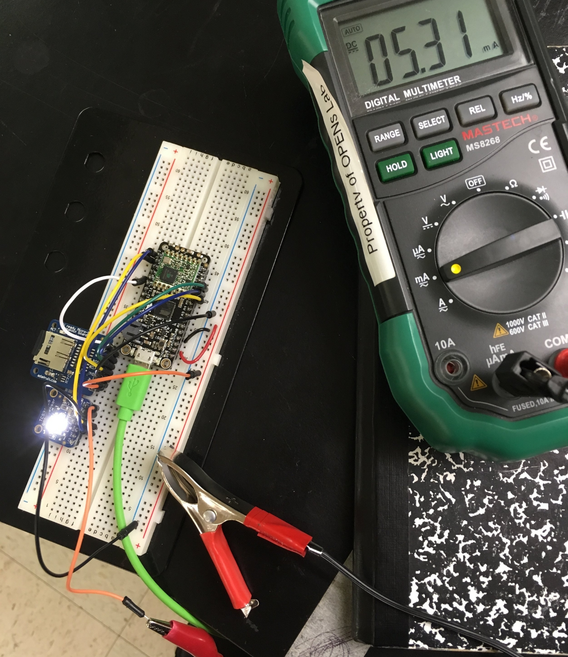
With the LED light powered on, the TCS34725 requires 5 mA of power to operate, making it an unfavorable candidate for long term deployment.
Evaluation of the TCS34725:
After testing Adafruit’s TCS34725 and running a current test, it was clear that the functionality and power needs of this sensor were not what we were looking for on the Evaporometer project.
A significant amount of power would be needed to read the RGB values and such data would be virtually useless in spacious outdoor areas. While lux, color temperature, and the visible spectrum could be used to compare data with our Evaporometer’s TSL2591 sensor, it also makes sense to integrate a second TSL2591 sensor or conduct a side-by-side comparison of the two sensors to see if programming the TCS34725 to only measure lux values requires less power than the TSL2591.
UPDATE: A Closer Look at TCS34725 Functionality
As I mentioned at the end of the previous section, I thought this sensor could be useful to us so long as we disabled the RGB color reading functionality and shut off the white LED to save power. After some digging around in the TCS34725 data sheet and TCS34725 library I learned a lot more about the full functionality of this neat light sensor – like many Adafruit sensors, this RGB sensor is capable of entering a low power mode that drastically reduces current consumption by only reading RGB color info at specified times. Unfortunately, I also found that forgoing measurement of RGB values also makes it impossible to calculate Lux (lumens per square meter). In this version of the TCS34725 library, lux calculations are derived from the RGB values of the light sensor, however this comment in the source code suggests that this may change:
The developers suggest using the clear (C) measurement to find lux – hypothesizing that doing so may improve accuracy. While the clear value is also measured in the same function that measures RGB values, it is possible an updated version of the calculateLux function and a well timed interrupt could also get the job done (using more power than our preferred IR/Full light sensor).
– Marissa Kwon, URSA and NSF Grant Summer Student Researcher
I have been putting together three power pulse controllers. One has already been sent out, but two more are in production. Here is a quick overview of the system specs and parts.
Methods:
I used Fusion360 for the modeling of the PPC and to create the 2D drawings so that other people can create it more easily.
Results:
Here is the model of the finished model on which everything was based off :
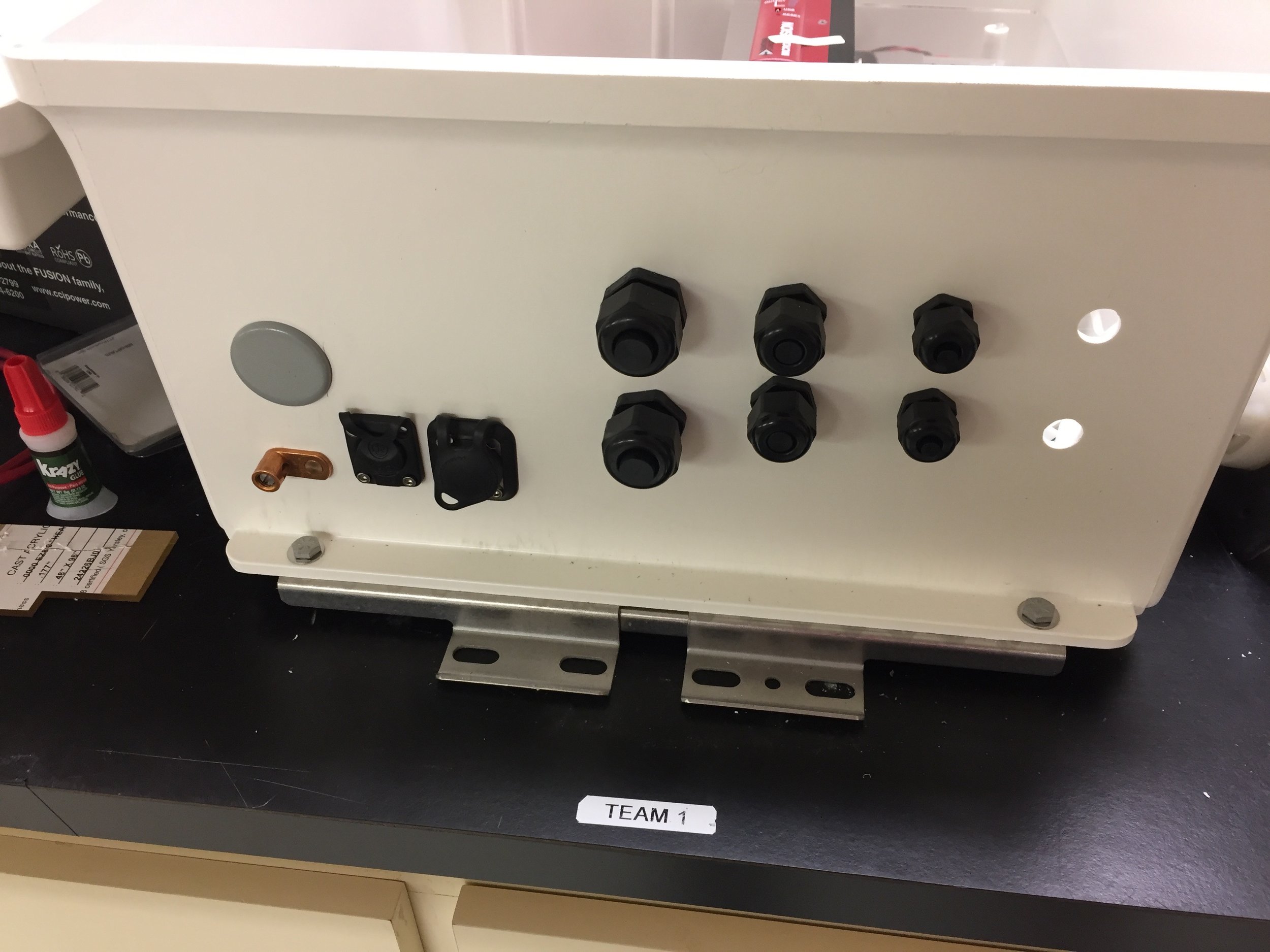
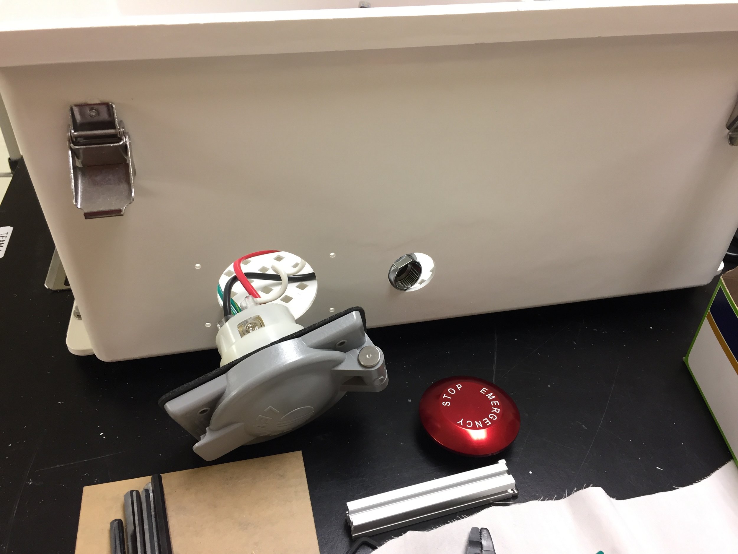
The 2D drawings (link above) contain the layout of the components on the backboard and the locations of the holes made for the components that go on outside of the enclosure. There are some extra components that are not modeled in the CAD that come with the enclosure. These are not modeled because we were not the ones who put them on there; our pieces do not interfere with these pieces.
Here is a picture of the extra pieces that come with the enclosure:
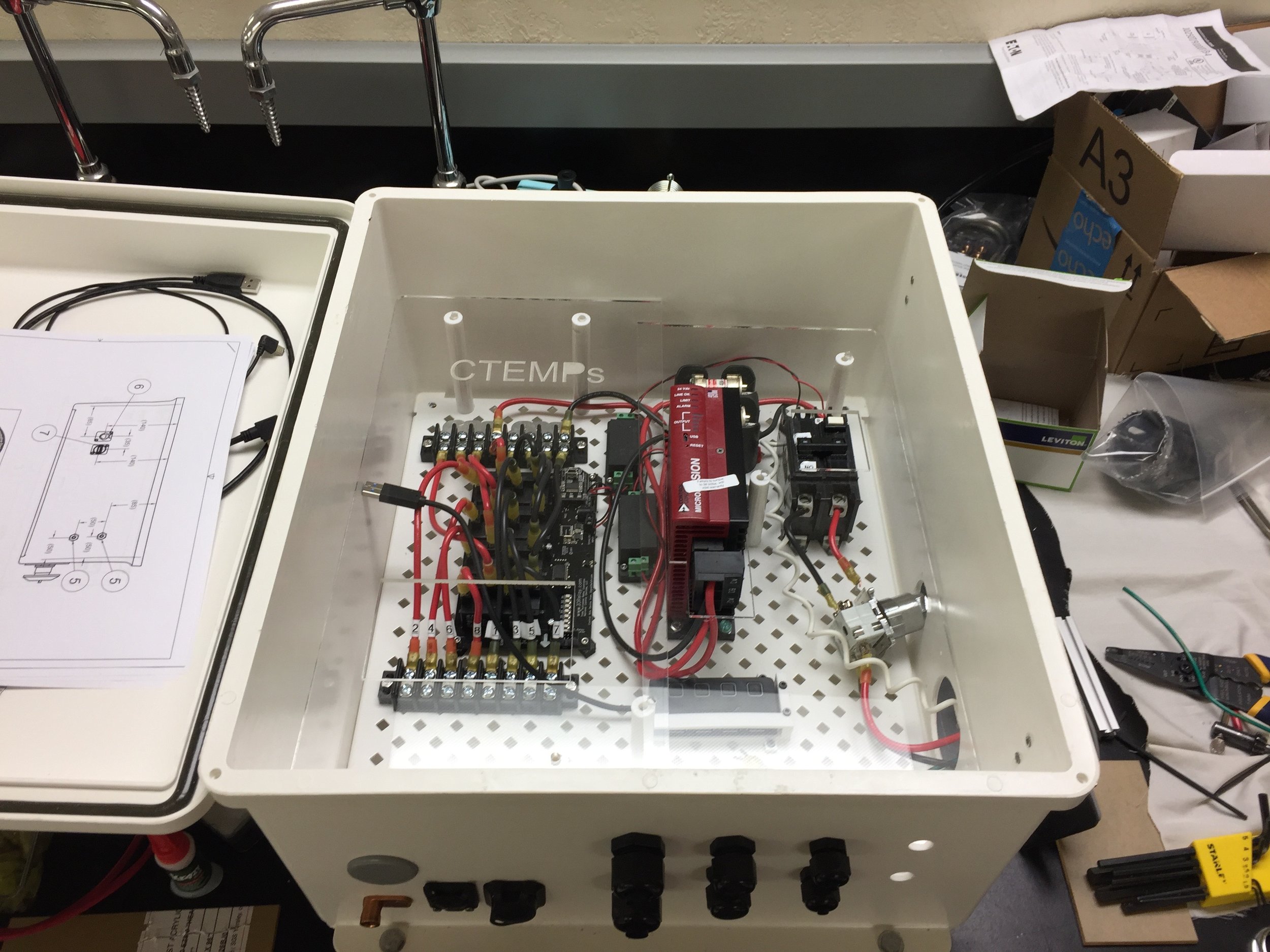
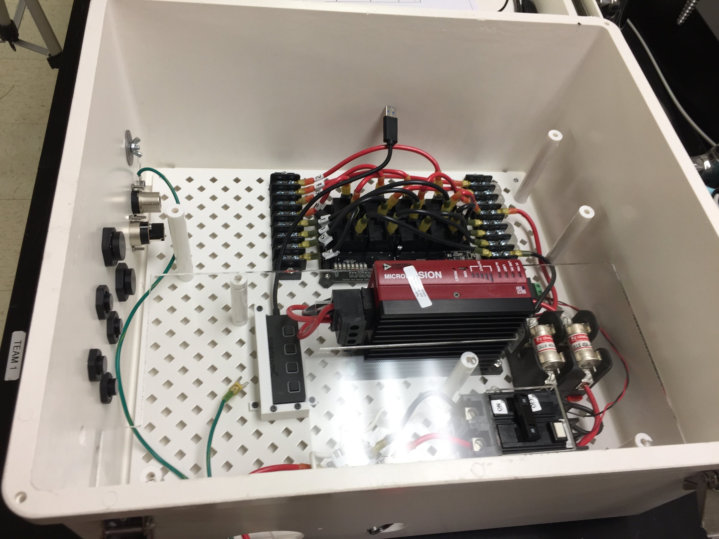
Here are other pictures of the other two Power Pulse Controllers being built:
The EPA recommends a flow rate of 2 ft./s or greater to minimize the relative difference in velocities of suspended sediments. They also recommend a tubing diameter of 1/4 in. as well, but not for a particularly well documented reason. One unanswered question brought up in the design review meeting was the impact of tubing diameter on the quality of water samples. This short writeup discusses some of the considerations involved in the decision to use 1/4” OD Teflon tubing for future sampler designs.
Design Considerations
A paper published in 1985 collected some data on this subject [link to paper]. It discusses several trials where different concentrations of dissolved organic compounds were passed through tubing of varying diameters and materials at a known rate. The concentrations of the passed solutions were measured and recorded.
There are two obvious factors involved: the tubing absorption rate and friction. Absorption is based on contact time, tubing area, tubing material, and the analyte. Absorption is not a concern in suspended sediments but is critical when the analyte is dissolved carbons and gases. Contact time is based solely on flow rate.
The friction coefficient is decided by the material and the force of friction will be proportional to the tubing diameter and flow rate. The force of friction will reduce the flow rate of the sample water, increasing contact time between the tubing wall and the sample water. Lower flow rates also reduce the accuracy of suspended sediment sampling where particle mass is a dominating factor that creates a differential velocity between the particulate sizes, shown by this study [link] mentioned to me by Dr. Babbar-Sebens.
The results of the experiment suggest the diameter of the tubing has a lesser effect than the material of the tubing on absorption rates for inner diameters between 1/4” and 1/2”, however increasing the tubing diameter decreases the absorption rate for the same material. This effect is unexplained in the paper and the relationship between tubing diameter and sample quality has very little research behind it. It is likely that the largest factor in choosing the tubing diameter is the maximum particulate size of suspended sediments, which requires a minimum diameter cross section throughout the entire hydraulic system including the solenoid valves and pump tubing.
Both the study mentioned above and this other study [link] show that teflon tubing absorbs the lowest proportion of dissolved organics. The EPA in this paper [link] also suggest that a high velocity decreases the slime buildup against the inner surface.
Conclusion
Because large suspended sediments (1mm+ diameter) are beyond the scope of the current sampler, Teflon tubing with a .17” ID and .25” OD will replace the current 3/16” ID Silicone tubing. Compression fittings will have to be used rather than barbed fittings. The change in diameter of the tubing will increase the velocity significantly and the teflon tubing will have much lower coefficient of friction, improving small particulate movement in sample water. Teflon tubing will be nearly impermeable to gases and will absorb extremely low amounts of dissolved compounds in the sample water, making it ideal for most of our intended applications, such as sampling for dissolved organics or volatile isotopes.
I have gotten the first prototype of the HyperRails working. I will be discussing the parts and setup.
Object:
This post is intended to update and inform about the progress with this project.
Materials and Methods:
We are using the V-slot aluminum extrusion and carriage system from openbuilds. All other parts were previously discussed in the last post about the HyperRails. These are the ones that are 3D printed in the lab.
All of the pieces were assembled according to the CAD. This step was pretty straight forward, the one that took more time was rolling up the line on the spool and tightening it on the carriage. This took more time due to the fact that the line would tend to get loosen up and some times tangle up while coiling up on the spool.
Results and Discussion:
Here is a video of the system in action:
The system works very well, we can see the movement of the carriage is very smooth.
Here are the links to the electrical components and code.
The main consideration for the next iteration is to make the system be able to work with all lengths. The main problem with this system is that the length of line needed for the system to work covers almost the whole surface of the coiling spool. After the line starts to overlap, the programming will have to be more complex to account for the decrease or increase of the diameter of the spool. This is the next problem to address with the next iteration. Our current system can only spool about 1.5 meters of line, and this system has to be designed to work will all lengths. One other consideration is the stretch of the line. When we were testing the system, in some cases we over extended the line and it would stretch a lot. I will need to find another fiber that has a very low stretch.
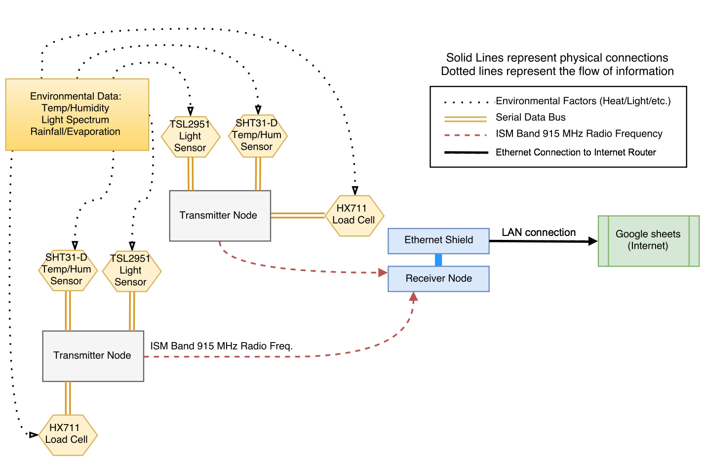
So far we have used this series of blogposts to discuss a lot of the technical details about how certain processes are happening within the Evaporometer Transmitter and Receiver. A series of diagrams has been made to help visualize how everything comes together. First will be a diagram showing how all the sensors are connected to the Feather 32u4 and battery, followed by two flowcharts illustrating how abstract environmental conditions are transformed into the data logged in our spreadsheet.
Evaporometer Transmitter Connections:
Pictured above is a very simple assembly diagram for the Evaporometer Transmitter. Notice that many of the devices have the same yellow and blue colored lines – these are the serial clock and data lines respectively and they are all hooked up to the same pins on the Feather. The red and black lines represent power and ground, and all devices must be connected to these nodes in order to receive power. In real life, the power and ground rails exist along the far edges of a protoboard or breadboard so that all the device wires do not need to be crammed into one small area.
Flowcharts Following the Progression of Evaporometer Data:
Sensors turn information collected from the environment into quantifiable values such as integer and float values that eventually get passed on to the receiver and logged onto a spreadsheet where we can see them online. The diagram below shows how data moves from one component to the next through the Evaporometer Transmitter. Each labeled point on the flowchart indicates where the data must undergo at least one change before being able to proceed to the next.
Although it may seem like a fairly simple process, the sensor data must undergo several transformations before it can reach its destination on the spreadsheet. The integer and float values collected by the sensors must be turned into strings so they can be concatenated into one long packet of data. Now as a single piece of information, the string is cast into an array of 8-bit characters so that it can be transmitted and received using the LoRa components built into our micro-controllers. When the message is received it must also be broken back into the same pieces before it was concatenated and able to be cast back into the float or integer values. To do this we add a comma as a delimiter placed in between data points during concatenation, and once it is received we use use strtok() to divide up our character array at the location of the commas to separate the packet back into different pieces of data.
The diagram below illustrates each process that takes place in the transmitter, starting with data collection right after the RTC alarm wakes it up.
– Marissa Kwon, URSA and NSF Grant Summer Student Researcher
The description of process of using PushingBox and the Google scripts was updated 10/3/18 (primarily with regards to the usage and interfacing with the Google Script). The most up to date and comprehensive tutorial is now maintained here.
Abstract
Connecting… Connecting… Transmission Received!
After months of prototyping, experimenting and redesigning we have successfully deployed our first, “fully open source” transmitter and receiver with near real time updates to a google spreadsheet. This post will give a step by step procedure on how to set up all the software and web interfaces for this project.
Step One – Creating and Deploying your Google Sheet
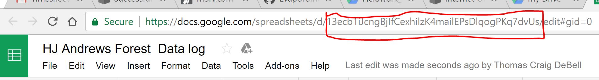
A) Log in to your free Google account and create a new “Google Sheet,” this is the spreadsheet which will be populated by the sensor data received by the Ethernet Featherwing data logger. At this point, you will need to copy and save your spreadsheets URL key for use in your Arduino code. This key is listed in the URL between the “/d/ ” and the “/edit ” of your new spreadsheet (see red box).
B) Name your Spreadsheet something original like “Environmental Data,” now we must create our Google App Script (similar to JavaScript) which will process our data and populate our spreadsheet correctly. To insert our Google App Script we first navigate from our spreadsheet to the Script Editor, found under the Tools tab:
Tools →Script Editor
We will now be on the Google Script Editor page. Now we can name our Gscript something extra-creative like “My Environmental GScript”, but do not have to. Fortunately, we do not have much that we have to do on the Script editor page.
1) Copy and Paste the Google Script code into the Editor. (link to GitHub with all needed codes here)
2) Save the script: File→Save All
3) Deploy as a web App: Publish-→ Deploy as web App…
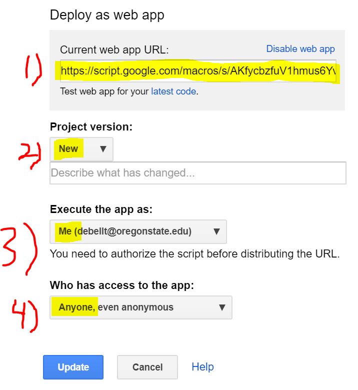
C) Our final Step for setting up our Google sheet will involve configuring the Web deployment parameters. It is important you set all these fields correctly. If you don’t set all four fields exactly your spreadsheet won’t work properly (trust me…). This step takes place immedietly after clicking “Deploy as Web App”.
Field 1) Copy and Save the “Current web app URL:“ which has just been generated, we will need this later when we configure our API in PushingBox.
Field 2) Save a project version as “new” on each iteration, it’s important to note that if you don’t make a new project version for each script revision you make (if you decide to make any revisions), your script revisions won’t be updated on the web. This is counter-intuitive, and easy to neglect, but this is currently how Google has this system configured.
Field 3) “Execute the app as: “ set this to “me(your GMail here) ”.
Field 4) “Who has access to the app: “ set this to “anyone, even anonymous.” *This is important, and allows Pushingbox access the spreadsheet.*
Step Two – PushingBox API
Pushingbox.com serves as simple, free, and easy Application Programming Interface (API) middleman in allowing our Evaporometer data to be palatable to Google Sheets. The need for using the PushingBox API intermediary is to turn our HTTP Ethernet transmitted data into Google compliant HTTPS encrypted data. Although other programmers have found workarounds to this system (found here) using PushingBox is easier, and we are given up to 1,000 requests (Data Transmissions) a day.
*1,000 push requests is more than enough for updates every 2 minutes in a 24-hour cycle but not enough for minute by minute updates (thus the “” around real time) but this service is completely free.*
Below are the steps for configuring Pushingbox to work with our data:
1. Create a PushingBox account using your Gmail.
2. At the top click on “My Services”
3. While now in “My Services” go to the “Add a service” box and click on “Add a service”.
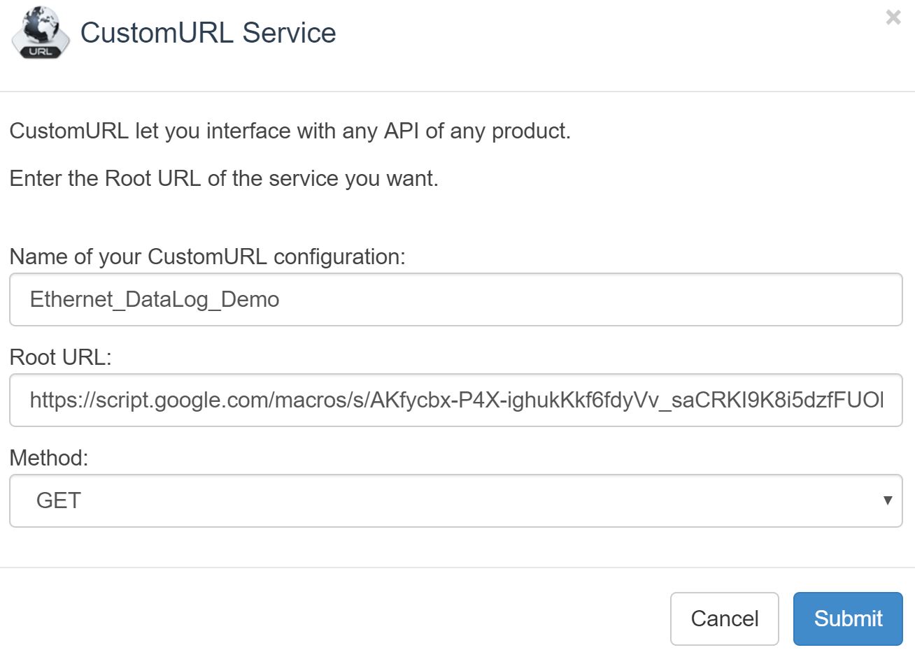
4. The service you will want to create is the last item on the list of services and is called: ”CustomURL, Set your own service !”. Now select this CustomUrl service.
5. A box will open up and ask for three items. Fill them out as below, then hit submit
Name of your CustomURL configuration:
Root URL:This url will start with https://script.google.com… as this is your Google Script address saved from Part 1
6. After submitting your service you must now create a scenario for the service. To do this select “My Scenarios” at the top of the page.
7. Enter an appropriate name for your scenario in the “Create a scenario or add a device” box. After you name your service click the “add” button to the right.
8. Now it will ask to “Add an action for your scenario” You should now choose the “Add an action to this service” button listed next to the service name you created in the previous step. This assigns your new scenario to your new service.
9. A data box will open asking you for your “Get” or “Post” method (we use the Get method although this seems counter-intuitive). For recording all our Evaporometer data into your Google sheet you need to link your variable names listed in your Google App Script to the names listed in our Arduino sketch. Formatting the names correctly in the Pushingbox API will accomplish this linking task.
Copy and paste the following string into your box.
?key0=$key0
amp;val0=$val0
amp;key1=$key1
amp;val1=$val1
amp;key2=$key2
amp;val2=$val2
amp;key3=$key3
amp;val3=$val3
amp;key4=$key4
amp;val4=$val4
amp;key5=$key5
amp;val5=$val5
amp;key6=$key6
amp;val6=$val6
amp;key7=$key7
amp;val7=$val7
amp;key8=$key8
amp;val8=$val8
amp;key9=$key9
amp;val9=$val9
amp;key10=$key10
amp;val10=$val10
amp;key11=$key11
amp;val11=$val11
amp;key12=$key12
amp;val12=$val12
amp;key13=$key13
amp;val13=$val13
amp;key14=$key14
amp;val14=$val14
amp;key15=$key15
amp;val15=$val15$
Note: STATEMENT BEGINS WITH ” ? ” TO INDICATE “GET”
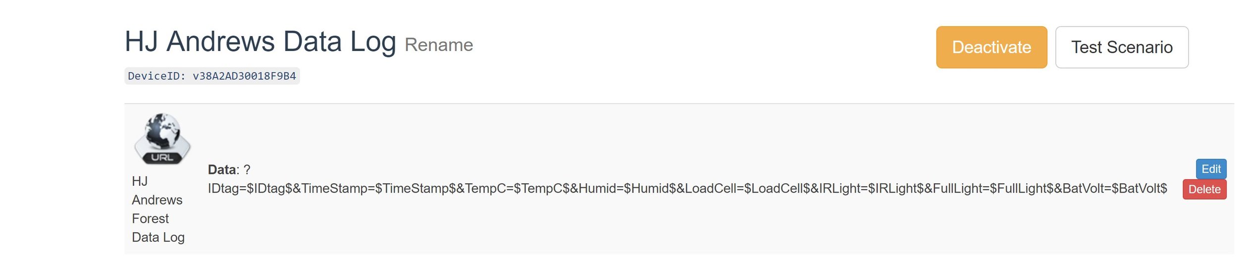
The result should look like as follows (roughly, as the data string shown in the image is slightly out of date, but the rest is correct), but with your own scenario name and Device ID number:
*Make sure to copy your “DeviceID” string that will be generated after setting up the service, you will need it for both preliminary testing in the next step, and later for the Arduino Sketch in Part 4.*
Step Three- Testing API and Google Spreadsheet
Before we move on to the last step, in which we program the Adafruit Feather 32u4 with LoRa Radio Module and complimentary Ethernet Feather Wing which will log data through the web, it would be helpful to test that everything we have done thus far is correct. If we wait to complete the hardware portion then the cause of any errors may be more difficult to track down. Fortunately, we have a simple method of testing our code so far. We can just directly enter some hard-coded pseudo-data into our web browsers address bar and check that our Google sheet is being updated correctly. Here is an example of what you might copy and paste into your browsers address bar.
If you like you can even re-enter new fake data with different values for subsequent rows, however, remember you only have a 1,000 requests per day from Pushingbox.com so don’t go crazy! If this procedure did not update your spreadsheet then go back and review Parts 1 -3 of this instructional for errors before attempting Part 4. Congratulations if you have made it this far, the worst is over! (it took me about a dozen times to get all the previous steps correct) Update – the modification of this process and the Google Script since the initial writing of this blog post were primarily to simplify these steps
Step Four – Hardware Set-up and Arduino Sketches
After confirming you were able to push some hard-coded pseudo-data directly from your browser onto your Google Sheet you are now ready for the next step which involves sending data directly from the Feather 32u4 and complimentary Ethernet Feather Wing to Google via Pushingbox over an Ethernet connection. Before you can upload and run the included Arduino sketch to the Feather Board you must complete the following three steps.
Hardware
1. Wiring the Feather 32u4 board to the Ethernet FeatherWing: a guide on how to do this can be found on the adafruit website here, as well as one of my previous posts, found here.
Software(1):
2. There are a few steps to set up your Arduino IDE to work with your Feather 32u4 board.. These steps include downloading the necessary libraries and configuring the Arduino IDE (1.6.4 or later) with the correct Feather Board package. Many of you will have already installed all the software you need, for those that have not, below are links to retrieve the needed libraries and the Feather 32u4 board support package.
The two required libraries for our particular sketch:
Two great tutorials to walk you through getting the correct Feather 32u4 board and Ethernet FeatherWing package installed into the Arduino IDE if you haven’t done this already:
3. You are now ready for the final step of the project, you need to copy and paste the included Arduino sketch, customize it for your device, and then upload the sketch onto your Feather 32u4 board and Ethernet FeatherWing. Update – that sketch is now out of date, refer to the Loom Library instead for the corresponding updated code and process.
A) Your MAC Address (Found in Ethernet packaging)
B) Your Static IP address (May need to be given by IT admins)
C) Your Pushing box Device ID (devid)
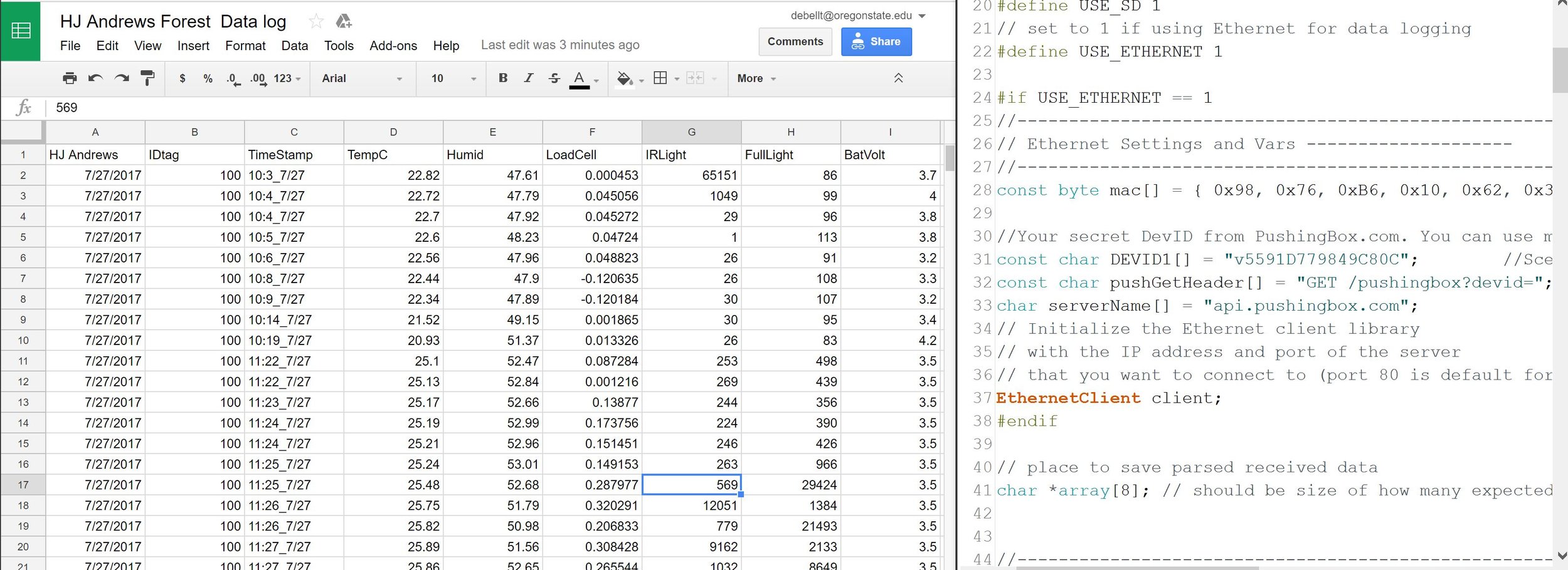
That’s it, you’re done! If everything was completed correctly your output will look something like the picture below:
Populated Google Spreadsheet (left) and Ardiuno IDE with example code.
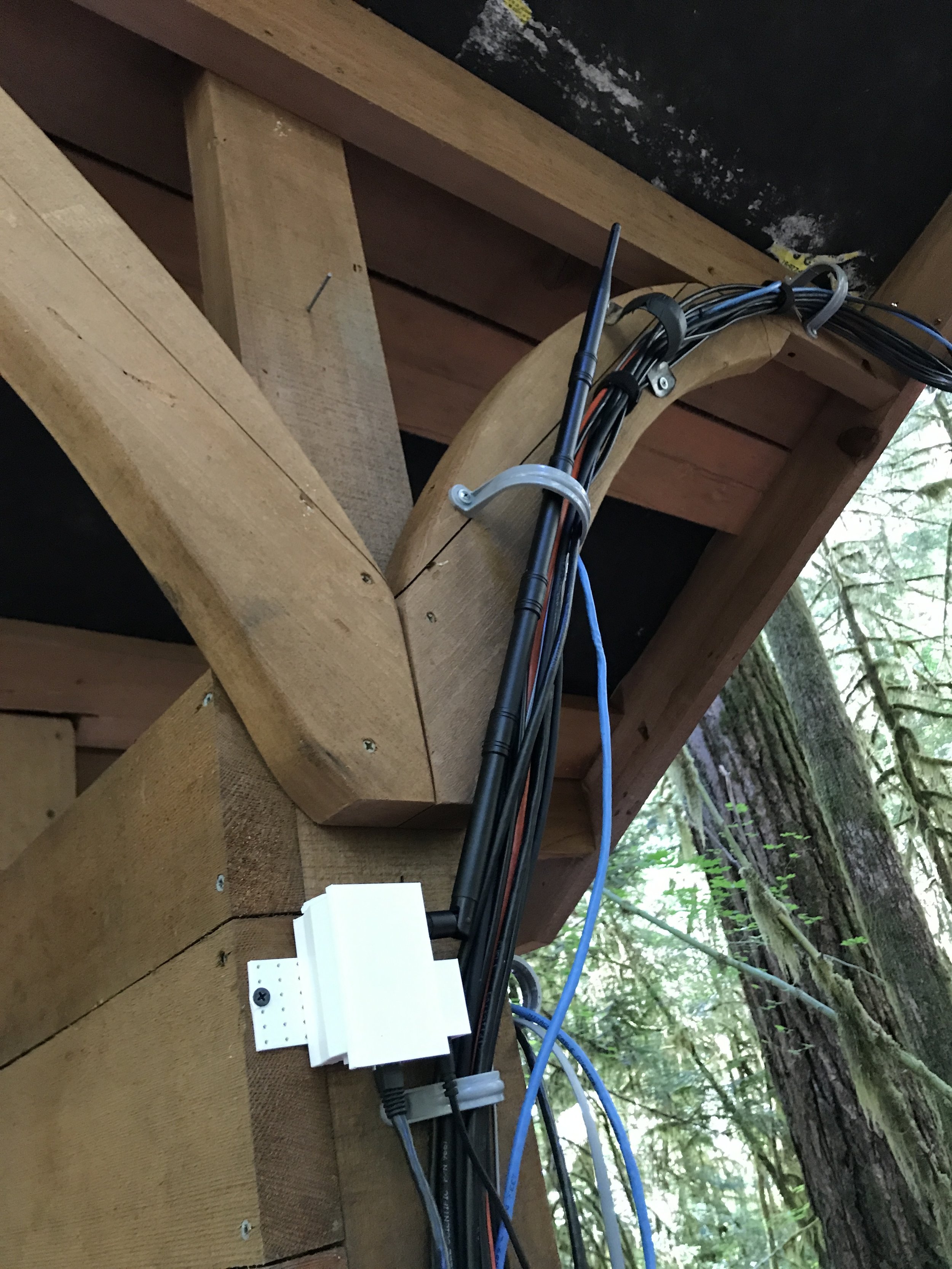
Final Receiver and Ethernet data logger set-up.
– Tom DeBell, Beginning Researcher Support Program Researcher
A bug in the water sampler’s electronics has come and gone throughout the iterations of our design: the valves would reset intermittently when the pump motor was operating. First we moved the pump from the same shift register as the valves to its own dedicated MOSFET. We added a small capacitor for mild noise. The problem disappeared until later iterations. Then, we changed the MOSFET to a dedicated H-Bridge motor controller from Adafruit, equipped with its own 22uF and .1uF decoupling capacitors. The problem disappeared until we used a larger pump in a later iteration. So we talked to Jim Wagner about it and he cleared things up for us.
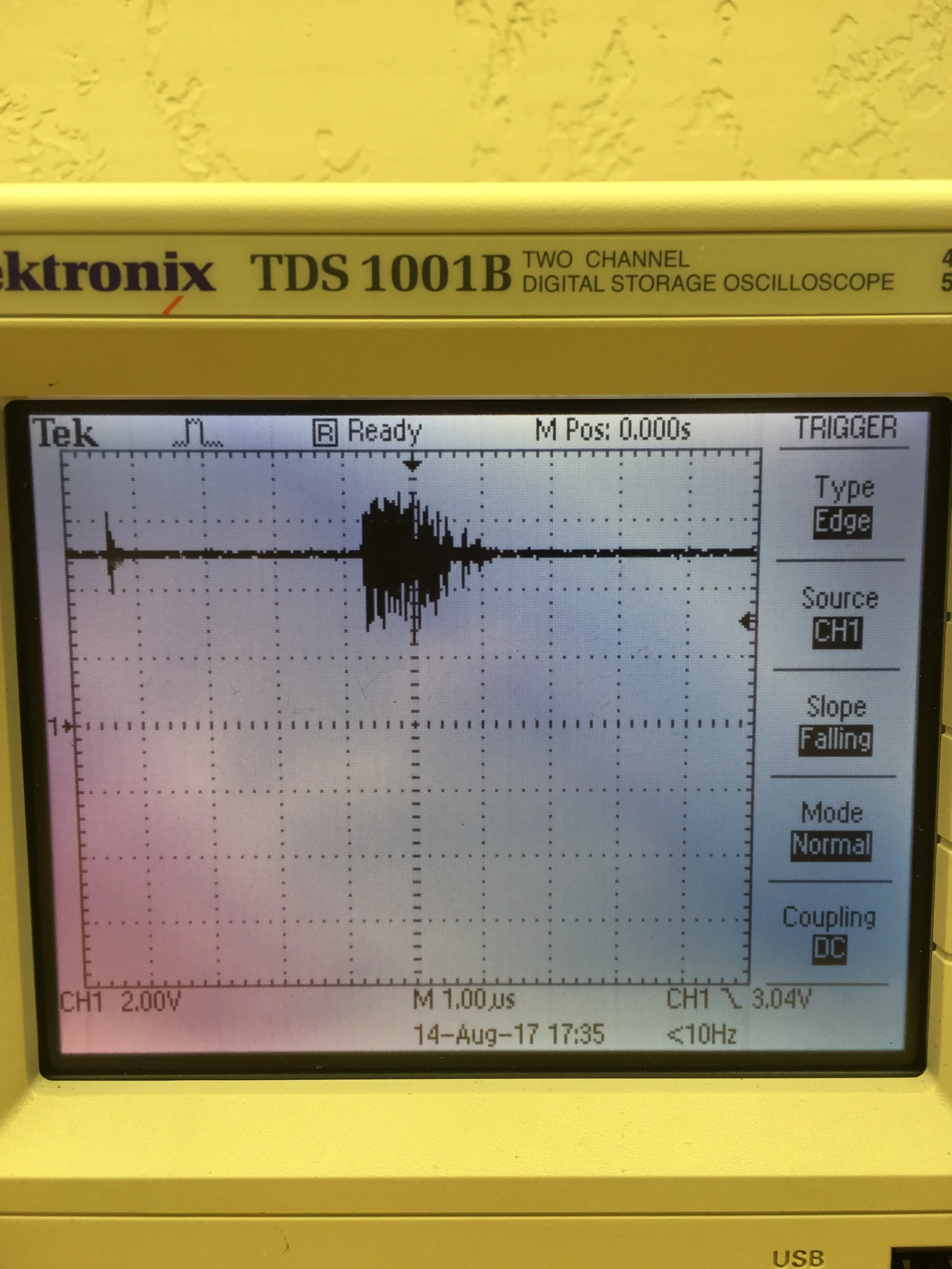
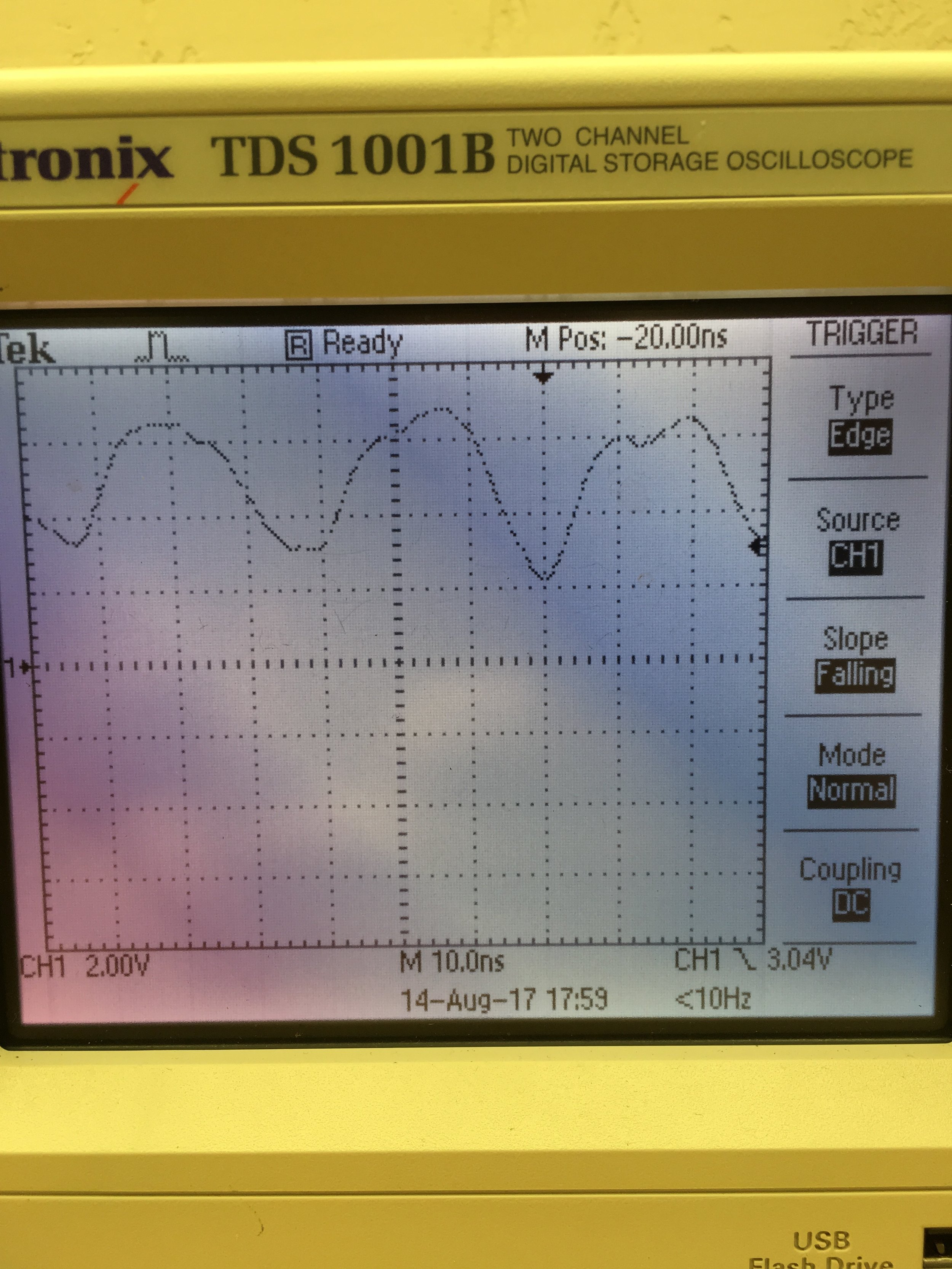
It turns out that brushed DC motors create a lot of noise, which is exactly as we expected but did not know how to fix. The brushes in the motors cause irregular noise in the power lines with pulse widths too small to pick up on a multimeter, but quite easy to see using an oscilloscope. I hooked up the arduino’s 5V pin and ground to a probe and ran the system under the conditions that would cause the valves to reset. The scope was set to trigger on a falling edge lower than 3.04v. Sure enough, the initially-open valve closed and water forced its way through the flush valve after building pressure.
Look a little closer at the oscilloscope:
The 5V rail dropped to nearly 0V for about a microsecond, more than enough time to drop the SCLR line to fall to a low state and reset the shift registers. This explains why the valves were resetting! It wasn’t just this one instance, either; the valve continuously reset as the command “V1 1” to open it was sent, and the oscilloscope was continuously triggering due to a falling edge like the one in the picture as long as the pump was running.
OK. We had already added a 100 uF capacitor between the Arduino’s VIN (12V) and GND pins. I removed that and bumped it up to 1000uF, reconnected the system to the oscilloscope and ran the test again, this time with similar but notably different results.
The valves were still resetting, and the oscilloscope was triggering often, but the voltage never dropped below 2V. A small victory, surely, however the problem remained. I decided to add a 100uF capacitor between the 5V and GND pins in addition to the capacitor that I had already attached between the 12V and GND. A retest resulted in the valves resetting after 8 seconds of stability, but the magnitude of the noise was still the same:
I read here after some quick research that multiple capacitors of different sizes in parallel would buffer different frequencies of noise. So I unplugged everything again and took the board to the soldering station, tacking on a 10nF ceramic capacitor parallel to the 100uF cap between the 5V and GND pins. This time the valves lasted 15 seconds before resetting on a much smoother blip, magnified to 250ns per division below:
The same signal magnified to 10ns per divison below:
So close! I carefully unplugged everything one more time, soldered on a 1nF capacitor in parallel, then set up the test one final time:
Finally, the valves stayed on! The system ran for a minute straight without so much as a whisper from the probed voltage. This solution can be used in the next iteration of the PCB after more research, calculation, and perhaps discussion with Jim in order to protect against a wider range of noise on more lines more efficiently.
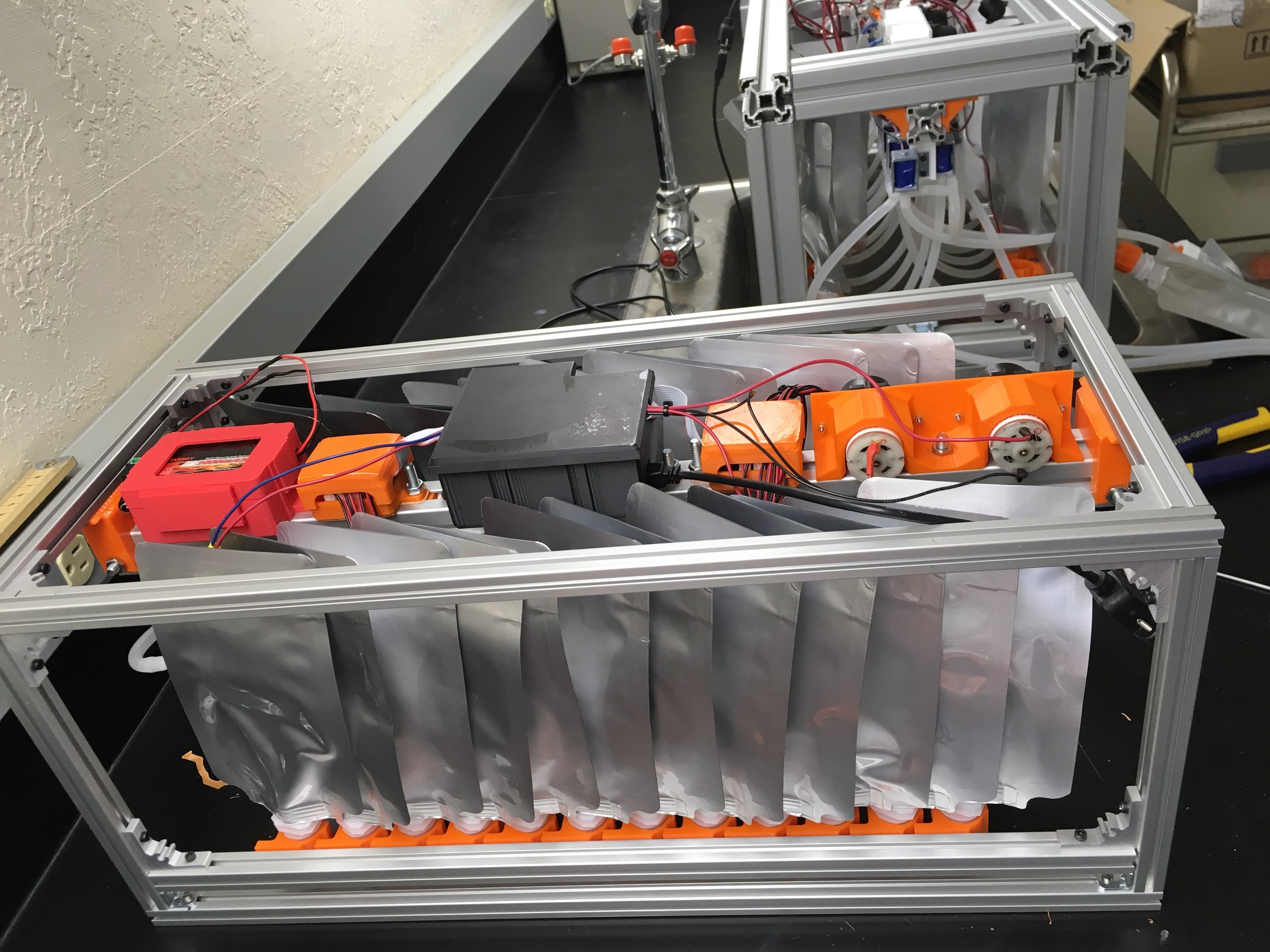
Much progress has been made with the OPEnSampler! The frame is lightweight, the entire system fits into the Pelican rolling cooler, and the sample control works as expected. 24 bags fit with room inside the frame, and the system can be set on any face without issues, easing maintenance, testing, transport, and drawing out samples. Some issues persist in this iteration, namely light leaking from the bags and a low flow rate due to the cheap pumps.
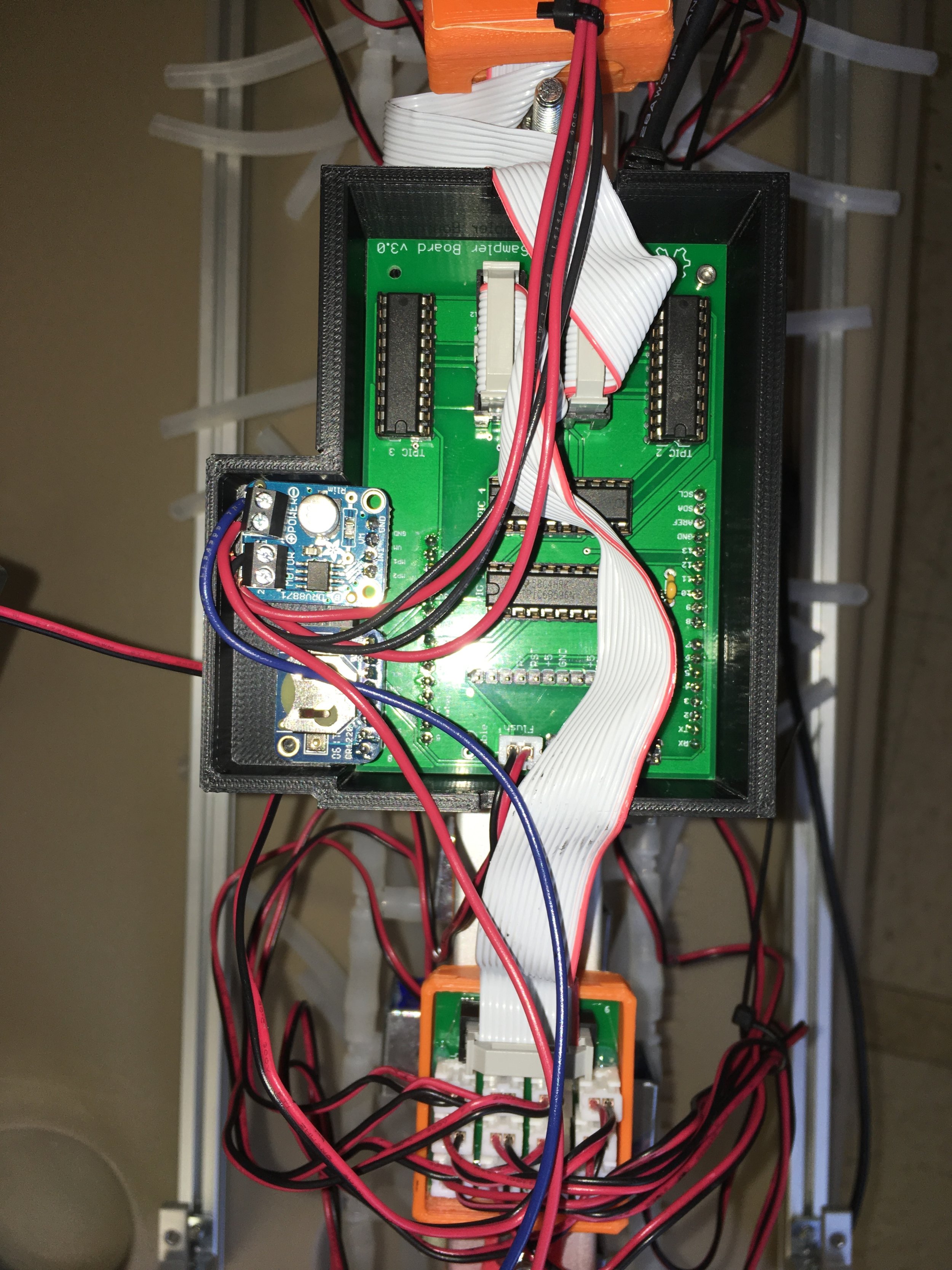
Electronics
The electronics of the sampler have evolved. They consist of an Arduino Uno connected to three custom PCBs: two Valve Breakout Boards (VBBs) and one Main Control Board (MCB). The MCB connects directly to the Arduino and includes the shift registers to control the valves, the motor breakout board for the pumps, the real time clock, and receptacles for ribbon cables connecting to the VBBs. The VBBs break out the open-drain outputs on the shift registers to 12 JST terminals each, corresponding to one valve each. Doing this reduced the wire-spaghetti caused by directly soldering wires to each valve.
Frame:
Slotted aluminum extrusion can be ordered at specific lengths with a tight tolerance for several dollars per piece, allowing the frame to be assembled in minutes with purchased corner brackets. A lighter but sufficiently strong 15mm aluminum extrusion was used, reducing the weight of the frame to just over 2 kg. The design of the frame allows the OPEnSampler to be tilted in any direction without issue.
Hydraulics:
Water to be sampled is pulled through an open end of 3/16” ID silicone tubing via two $12 peristaltic dosing pumps in parallel. The pumps claim to have a head height of “10m” and a flow rate of up to 150 ml/min, but in practice the numbers are about half those values. Further testing will be carried out, but the pumps will be replaced with a $60 peristaltic pump from a more reputable company supposedly capable of a 350ml flow rate.
Down-line of the pumps water fills the rest of the tubing, leaving the exit end if the flush valve is opened, or is pushed into a sample bag when its respective valve is opened. To draw sampled water out of a bag, its respective valve is opened and the pumps are powered in reverse using the H-bridge motor breakout board bought from Adafruit.
Current Bugs
There are a couple known bugs in the system and one major design flaw that limits the functionality of the device. The first bug is mechanical: the bags leak when they are upside down. Initially, this was a very significant amount, draining the bags overnight. Teflon tape was wrapped around the elbow connectors that screw into the printed bag caps, and the leaking was reduced to a few mL per hour. Initial tests of new bag caps with changed O-Ring gland dimensions, a 3% smaller diameter through-hole for the elbow fittings, and the replacement of teflon tape with a gorilla-glue and acetone coat show very promising results with no leaking in the first two caps tested. 24 new caps were printed, processed, and are currently drying before testing tomorrow morning.
The second bug is intermittent and will be difficult to fix. On occasion, valve 7 becomes permanently powered and will stay open regardless of what serial commands are fed to the Arduino. This is characterized by a lack of actuating sound when the command “V7 1” (valve 7 on) is sent, by bag 7 filling despite sending the commands to fill another bag, and by an actuating sound upon powering on the device. This bug is not consistent and the cause is currently unknown. Battery power was suspected initially, but when probed the battery read a high 12.7 volts.
The major design flaw is the low flowrate of the pumps, including the new pump selected. The EPA recommends a line velocity of greater than 2 ft/s when sampling for suspended solids such as sediments (link). With 3/16” ID tubing, this equates to a flow rate above 600 mL/min. Low flow pumps were chosen because high-flow peristaltic pumps cost between several hundred and several thousand dollars. A 3D printed pump head with a store-bought DC gear-motor is being investigated, though a <$100, 1000ml/min 12V pump has been found on AliExpress and will be tested out before a DIY pump is developed.
Conclusion
While a significant portion of this writeup was dedicated to discussing the current issues with the device, the OPEnSampler is working almost exactly as expected. If a solution to the leaking problem is not found soon, the bags can simply be reoriented to sit upright for this current version. The pumps will be sufficient in sampling for analytes that aren’t large-particle suspended sediments.