Abstract: Here is an update on the new evaporimeter design. This design will include the ETA sensor on it. It has not yet been designed, but the electronics base has the port for it.
Objective: This post is intended to update the reader on the new design for evaporimeter.
Results: The following CAD are the main pieces that make the new evaporimeter design.
This is the main body that holds the battery and the electronics. The battery sits at the bottom of the case and the electronics sit on top of the battery supported by a 3D printed base.
This piece is the on that holds the electronics in place. The bottom PCB is bolted onto this piece; this one is specifically designed to bolt the Feather RTC and uSD card wing.
This is the cap that will close the case. This is designed to be modular in height for 3D printing. Our electronics are made so that more capabilities can be added after production; this is done by stacking other shields onto the existing boards.
This is the assembly of the case without the cover. The aluminum piece extruding from the side is the strain gauge and the black piece is a cordgrip used to pass a cable with four conductors that will be used to communicate with the light and humidity/temperature sensors.
Much has happened with the samplers in the past two weeks! There are two categories of updates: those relevant to the Zurich Sampler and those relevant to the new versions of samplers. In short, the frames have been assembled for the new samplers and the PCBs are being soldered up; the new pumps arrived; the final pieces of the Zurich Sampler are coming together and it will be ready to ship very soon.
Updates:
New Sampler Updates:
Frame:
The sample-bag OPEnSampler frame was assembled by Adnan and I the other week and it fits snug in the Pelican 80QT rolling cooler. It fills up quite a bit of the space as intended, and there is extra room on the sides (the thickness of the wheel wells) for ice packs. Before more are assembled I think I will reduce the width of the sampler by about 5mm to account for the wells being slightly convex.
PCBs:
The Main Control Boards arrived the other week along with all the components of the two samplers. They look great! Azad and Adnan are soldering the components to them and will likely finish in a couple weeks.
New Pumps:
The new pumps arrived and we will be testing them soon. It looks proming but we will need to change either the tubing or the tube fittings to work with the rest of the sampler tubing. These will be added to the new samplers Azad and Adnan are assembling.
Android App:
In other news, three students will be working on adding an Android app to receive updates from and control the sampler remotely as their senior capstone project for their majors in computer science. In the coming weeks they will be contributing to the blog by introducing themselves and eventually posting updates on their work on the app.
Zurich Sampler Updates:
Quick Disconnect Fittings:
I finished the design of the endcap on which the two quick disconnect fittings are mounted and it is currently printing. Designing the endcap was more of a challenge than I initially predicted due to the awkward nature of the barbed fittings and the Pelican’s small outlet port. Because the threaded outlet on the Pelican cooler is too small to fit two fittings side-by-side, the endcap was designed in two pieces that would clamp together with an o-ring and three M2 screws. The male fittings can be threaded through the front panel with an o-ring to mitigate airflow. The sampler tubing can be pushed through the main body of the endcap while it is disconnected from the front panel, and then attached to the barbed ends of the fittings. The main body is then screwed onto the Pelican’s outlet port and the front panel is attached to the main body via M3 screws and nuts, completing the assembly. Intake tubing is attached to the intake fitting via the female quick disconnect fitting.
Filter:
The optional filters were quite easy to integrate into the design. The filter mesh is 470 micron stainless steel from Grainger with open ends. The front of the intake is blocked with a simple 3D-printed plate and the other end is blocked with another plate with a compression fitting screwed into it. All components of this assembly are glued with “ABS paste”, a solution of dissolved ABS plastic filament in acetone. The paste acts to weld the plastic components together.
Operator Interface:
The new Operator Interface turned out quite well. It consists of a 12V barrel jack port for powering the device with either a battery or a voltage regulator, a power On/Off switch, an enable switch for changing sampler modes (field use vs lab testing), an interrupt override button for initiating sampling in the field and also for lab testing, and a USB type B socket for communicating to the Arduino with a laptop. The panel is 3D printed and slides into the 15mm extrusion.
Conclusion:
There’s a ton of development happening on the OPEnSampler and I’m excited to showcase the new design once the two new samplers are completely assembled. In the coming weeks we will ship out the OPEnSampler for the first time, I will update the gitHub page with the latest designs and bill of materials, the capstone students will introduce themselves on this blog, the new pump will be tested, and the new samplers will be fully assembled.
One problem that I’ve been having with burying the Smartrac Dogbone tags is that soil is that they break after some use. After taking a close look at some of the broken tags it appears that this is caused by the abrasive soil eventually cutting through the outer lamination of the Dogbone tags and then damaging the IC that controls the tag, causing them to become unresponsive. To counter this, I designed a two part protective enclosure for the tag that will hopefully protect them from damage. The design is outlined below:
This “Dogbone Sandwich Shield” is made up of two identical 3-D printed parts. The sandwich ends were designed to be slightly larger than the Dogbone’s footprint with two tabs on the long ends. The tabs were placed like this to minimize interference with the moisture sensitive area of the tag which sits at its center.
Assembling the product was a fairly simple process. First, the Dogbone tag was stickered onto one of the sandwich ends. Then a small amount of acetone was brushed onto all of the sandwich end’s tabs. They were then pressed together to create a sandwich with the Dogbone in the middle. The sandwich was then treated in an acetone air bath to seal the edges. After 20 seconds in the air bath, the part was removed and put in a vice under a small amount of even pressure to make it even until it hardened. It takes around a day to fully harden, but it is tough enough after an hour. Below is a picture of the final shield.
Results
The presence of the shield surrounding the Dogbone tag made it slightly less sensitive to moisture, however, the variance from readings with the shield was no greater than it was without them. Therefore, using the shield will not influence the accuracy of the sensor once, but it will require some re-calibration.
Thinking Ahead
Thinking ahead, creating shields like this one with varying thickness could allow for changing the sensitivity of the tags. Currently, without a shield, the tags read their lowest value before the soil has gotten completely saturated and are able to read soil that is more than completely dry. Adding a shield that is a certain depth should shift the reading range to be centered and allow the tags to read over a larger range of soil conditions than they currently do.
Abstract: It was recently discovered that our transmitter is no longer sending data and that the last reading on the humidity sensor was 100%. I wonder what happened? We are now moving ahead in the design process to create a waterproof system.
Objective: I intend to describe design considerations and current ideas that have come up to design the new enclosure for the evaporimeter base.
Materials and Methods:
This the new concept for the evaporimeter:
The idea of the new base is to have a case that consists of a main body and cap. I think it is a good idea to use a rubber gasket to seal the junction between the two. In terms of materials, I plan to keep on using ABS for the time, but using T-Glase, Bridge, or Nylon is also recommended to keep water from entering into the 3d printed case.
We also need to run some wire into the casing from the sensors on the outside. Using a coupling mechanism would be our best solution. The only problem is that our system is very small and the coupling mechanisms for that scale are very expensive, about $40 per set. Another solution that was brought up was to use rubber sheet and perforate a small hole to run the wire through. This rubber sheet will seal up against the wire and keep moisture out. We are also leaning towards using a cordgrip and using a 4 wire cable. Another solution was to find some type of waterproof ethernet cable.
Results
For now, we will be testing the cordgrip and ethernet options. These seem to be the most inexpensive options. I will also be ordering the rubber gasket to get a good seal for the base case.
Over the last two months, our OPEnS Data logging hub in the HJ Andrews forest has relayed over 100,000 data points to our Google Spreadsheet through the transmission protocol below. This post will provide a brief look at some interesting trends found within our dataset.
Data Transmission Diagram
Objective
The Objective of this post is to look at some POI within our data set including some interesting plots of data during the Great North American Eclipse.
Data
After collecting data points every 5 minutes for a little over two months we were fortunate to begin looking at the wealth of valuable data we had collected. As I began to analyze specific areas of the data that I found interesting, I was able to see some pretty fascinating trends that one would expect to see such as the Inverse relationship between relative humidity and temperature. I then began exploring other trends within the data and found that although some trends were expected some were not.
Graph showing the inverse relationship of relative humidity and temperature
It became clear after looking at the load cell data (well after all water we added to the system would have evaporated) that there was a periodic fluctuation much greater than any residual noise would account for. When plotted alongside daily temperature, it was clear that fluctuations were temperature dependant and we deducted that the exposed aluminum force gauge was expanding with high afternoon temperatures and contracting with colder overnight lows. This behavior visible in the graph below.
Our data is not without its issues, We found our load cell (evaporation mass) data was greatly compromised by the thermal expansion properties of the aluminum rod throughout daily temperature fluctuations.
All issues aside, we were able to capture some pretty remarkable data during the Great North American Eclipse on August 21st, the below plot focuses on the point of totality, and how this event altered the standard linear trend of light intensity increase throughout a morning with a very steep fallout in both the Infared and Full spectrum light intensity. This anomely can be viewed below.
Light Intensity Data during the Total Eclipse 8/21
Conclusions
After briefly looking at the data from this spreadsheet it clear that a more in-depth analysis will be required to really gain an understanding of the relationships and trends within the data set. However, even at a glancing look, it is clear from the strain gauge and temperature relationship will be a major consideration in the redesign and further models of our sensor suites.
An alternative to the previous Honlite 1000mL/min peristaltic pump was required: our department cannot buy from Aliexpress or Alibaba, and Honlite only sells their pumps on those sites. Luckily, I found a 24DC, 2200mL/min pump for $99 on Amazon! Let’s discuss why this is a big deal and how it will work.
Discussion:
Peristaltic pumps generally come in two categories: cheap with a low flow rate, and extremely expensive with a high flowrate. Perform a simple google search for “high flow rate peristaltic pump”, and you’ll quickly realize why the first design tried to get away with two $12 pumps in parallel. On top of this, high flow rate pumps often require greater supply voltages or even an AC current not compatible with the current electronics.
The 2200 mL/min pump, despite its 24VDC rating, has a very affordable price for the specs. The 2200 mL/min is over 4 times the minimum requirement of 530 mL/min, based on the EPA’s recommended line velocity of 60cm/s or greater (source) and our chosen tube ID of 0.17” or 4.3mm. The manufacturer, in an answer to a customer’s question, said the user should expect their pump’s flow rate to increase linearly with supplied voltage. Based on this, we could expect the pump to provide a flow rate of roughly 1100 mL/min when powered from our system (12VDC).
Other Considerations:
The new pump comes with barbed fittings on either end of its soft tubing that are too large for the teflon tubing ID of 0.17”. Barbed x Compression fittings are an awkward, hard to find (possibly non-existent) kind of fitting so instead a Barbed x Barbed reducing fitting should be purchased. US Plastic doesn’t stock anything close to what we need, but two of these 3/16” x 3/8” stainless steel fitting from KegWorks should do the trick since 3/16 is 0.1875.
As our projects continue to evolve alongside with the advances of technology it is important to keep the OPEnS lab up to date with the latest and greatest prototyping technologies at our disposal. There is no example greater than that of the microprocessor. This post will explore two of the most advanced, widely available microprocessors on the market today.
Background and Objective
Since 2010 the Arduino Uno has been the standard in prototyping electronics due to its wide variety of functions, ease of programming, and cost. However, much like any other piece of technology it is becoming outdated by faster, smaller and cheaper microprocessors such as the pro-trinket model released in 2014. (A previous article I wrote linked here highlights the key advantages of the Trinket over the Uno.) Fast forward to early 2016 to the release of adafruits most current line of development microcontrollers, called “Feathers” with a host of companion shields referred to as “Featherwings“, where these processor boards now come integrated with certain features such as WiFi connectivity, Bluetooth, LoRa radio and Shields that allow for RTC data logging, Ethernet connectivity and various display interfaces. The Objective of this article is to discuss the two major types of processors used within the Feather line of microprocessors.
Materials and Methods
Featherwing 32u4 v.s Featherwing M0
Which is best? Well, it depends on a host of things. To begin let’s start with a side by side comparison with specs, cost and common troubleshooting problems that I and others in the maker community have encountered. Differences I found especially imporant are denoted with an *.
At the Feather 32u4’s heart is at ATmega32u4 clocked at 8 MHz and at 3.3V logic, a chip setup that has long been tried and tested. This chip has 32K of flash and 2K of RAM and is very comparable of that of a basic Arduino Uno (excluding the use of EEPROM memory).
At the Feather M0’s heart is an ATSAMD21G18 ARM Cortex M0 processor, clocked at 48 MHz and at 3.3V logic, the same one used in the new Arduino Zero. This chip has a whopping 256K of FLASH (8x more than the Atmega328 or 32u4) and 32K of RAM (16x as much)!
Measures 2.0″ x 0.9″ x 0.28″ (51mm x 23mm x 8mm) without headers soldered in
Light as a (large?) feather – 4.8 grams
ATmega32u4 @ 8MHz with 3.3V logic/power*
32K of flash and 2K of RAM*
3.3V regulator with 500mA peak current output
You also get tons of pins – 20 GPIO pins
Hardware Serial, hardware I2C, hardware SPI support
7 x PWM pins
10 x analog inputs (one is used to measure the battery voltage)
Built in 100mA lipoly charger with charging status indicator LED
Pin #13 red LED for general purpose blinking
Power/enable pin
4 mounting holes
Reset button
Long Battery Life*
From a purely technical perspective, it is clear that the ATSAMD21G18 ARM Cortex M0 processor is a superior processor in nearly every regard. However, running such a robust processor comes at the cost of power consumption which is likely an important factor in the design of whatever project you are looking at.
Ease of use and support
While specs are an important aspect to consider when selecting which type of feather you are going to work with another key component is the technical support available for the device. Like any new piece of technology, these adafruit products are not without their pitfalls, manly in the support of preexisting header libraries. I have found in my personal experience that the 32u4 model of the feather which uses an older processor found in many Arduino products has much more firmware support and has the ability to repurpose existing Arduino sketches much easier than with the M0.
The ATSAMD21G18 ARM Cortex M0 processor is much newer and more robust, which comes with the issue of not YET having support for many of adafruit and Arduino libraries. However, if your project doesn’t rely on interfacing with pre-existing technology or have dependencies on the old software you will probably be fine.
Discussion
In short, if you are doing projects that otherwise would have been prototyped on a device like an Arduino that doesn’t require a lot of processing power or large complicated scripts and battery consumption is of importance, the best choice would be the Feather32u4.
For more sophisticated projects that don’t require a lot of external dependencies, and for those with a strong background in computer and microprocessor programming, the feather m0 with ATSAMD21G18 ARM Cortex is a workhorse that allows for some pretty sophisticated programming with an abundance of memory and processor speeds.
Troubleshooting Some Common Problems
I “did something” and now when I plug in the Feather, it doesn’t show up as a device anymore so I cant upload to it or fix it…
No problem! You can ‘repair’ a bad code upload easily. Note that this can happen if you set a watchdog timer or sleep mode that stops USB, or any sketch that ‘crashes’ your Feather
Turn on verbose upload in the Arduino IDE preferences
Plug in feather 32u4/M0, it won’t show up as a COM/serial port that’s ok
Open up the Blink example (Examples->Basics->Blink)
Select the correct board in the Tools menu, e.g. Feather 32u4 or Feather M0 (check your board to make sure you have the right one selected!)
Compile it (make sure that works)
Click Upload to attempt to upload the code
The IDE will print out a bunch of COM Ports as it tries to upload. During this time, double-click the reset button, you’ll see the red pulsing LED that tells you its now in bootloading mode
The Feather will show up as the Bootloader COM/Serial port
The IDE should see the bootloader COM/Serial port and upload properly
Azad and I spent part of the morning assembling the frame of the bottle-based OPEnSampler. I found quite a few changes I will make when assembling the next sampler. In the end we found the device didn’t quite fit in the duffle bag and so some machining will need to be done to reduce a couple dimensions.
Assembling:
The assembly of the frame was a simple but tedious process. There were only a few unique parts: two different lengths of 15mm square aluminum extrusion, aluminum brackets, M3 screws, and M3 square nuts. The aluminum extrusion was cut by the manufacturer to specified lengths to skip right to the assembly stage. Azad and I each assembled an end face and attached a long extrusion, though it would have been easier to attach all the long extrusions to one face first and then attach the other face afterwards.
We found that attaching all the brackets at once to an extrusion resulted in sliding and flopping brackets while joining the opposite end to the frame; I’ll be sure to write the instructions so that brackets are attached only when necessary to avoid headaches. If that was unclear, most of the problems can be summarized as not attaching brackets when we should have attached them.
Fitting into the Bag:
Unfortunately I failed to dimension the frame to fit into the bag opening, which is slightly smaller than the bag space itself. Additionally, the height and length of the sampler were a bit too large to fit in the space anyways, so tomorrow I will have to disassemble the frame and head down to the machine shop to reduce a couple dimensions. Luckily it is easier to reduce the size of the device than to expand it, and there seems to be plenty of space for the bottles if I remove the ice tray from the design.
The spatial and temporal distributions of CO2 at the earth-atmosphere interface and at the boundary layer above it are of great importance for soil, agricultural and atmospheric changes. In general, the source of elevated CO2 concentrations at this boundary layer depends upon root respiration and soil microbial activity (Blagodatsky and Smith, 2012; Buchner et al., 2008; Nakadai et al., 2002).
Improvement of CO2 gas concentration detection could lead to a better understanding of the agricultural cycle and the transport mechanisms at this critical interface. Moreover, better monitoring methods to detect CO2 concentrations can provide improved modeling and decision-making to enhance agricultural productivity. Until recent years, the techniques for detecting CO2 concentrations included only stationary sensors that give close-range readings or the use of remote sensing platforms, which have limited accessibility due to their high costs and relatively low resolution (Toth and Jóźków, 2016). In addition, the use of remote gas sensing is usually inapplicable inside greenhouses.
The growing use of open open-source hardware (e.g., Arduino) for research purposes creates new opportunities to bridge the gap between CO2 detection at high resolution and affordability. In agriculture, the use of open-source hardware and sensors for CO2 gas sensing is still novel with little supporting research. However, recent research has revealed the possible applications of operating such gas sensing systems for agricultural purposes. For example, the use of an open-source gas sensing device to detect CO2 concentrations in a rectangular greenhouse (106 m × 47 m) was recently proven by Roldán et al. (2015). Using a low-cost electrochemical CO2 sensor, they provided a high-resolution CO2 concentration map inside a greenhouse. Their device also had temperature, relative humidity (RH) and luminosity sensors. All of the data from these sensors can be used for better greenhouse operation decision-making..
The aim of our research is to evaluate CO2 concentrations and dynamics using new CO2 (NDIR technology) and O2 (UV technology) sensors inside a greenhouse. We aim to integrate these gas sensors, together with temperature, RH, and luminosity sensors, on a single logging device to gain high spatial and temporal resolution of the greenhouse environment. In addition, we aim to make the device small and transportable to eventually deploy it on a drone or a rail system to get location-tagged data throughout the greenhouse.
2. Materials and Methods
The sensors used in this project are detailed on Table. 1. All sensors were chosen according the following guidelines:
(1) Sensor accuracy similar to that of a laboratory sensor. For example, the CO2 sensor should have the same accuracy range as other CO2 sensors that were reported in recent published studies.
(2) Only off-the-self, open source sensors.
(3) The sensor should be low-cost compared to other existing sensors.
(4) Only sensors that are modular and light-weight, such that the complete system will be light-weight.
Table 1. Details of the device sensors. The “Name/Model” column includes links for each sensor’s web site. Total cost of sensors (without the optional GPS Logger Shield) was less than 300 $.
[ coming soon ]
3. Results and discussion
System integration included all the sensors detailed in Table. 1. Picture of the device and connection scheme are detailed in Fig. 1-A and B, respectively. Two power connections were tested: a 9V battery and a fix connection to wall power using a 9V adapter. The advantage of using the 9V battery is the mobility of the device; however it was sufficient only for ~5 hr when logging data at 5-min intervals.
Fig. 1. Device description, (A) a photo of the device in the laboratory, (B) connection scheme of the different sensors.
To test the device, data was logged for six days in the laboratory (Fig. 2). Overall, measured parameters were as expected. During daytime the temperature was higher than nighttime with lower RH values. Correlation was observed between the working hours in the laboratory (08:00-17:00) and the peaks in luminosity and CO2 measurements. Once the first laboratory member entered the laboratory and turned on the light, we observed a corresponding increase in the luminosity sensor data. In addition, the CO2 in the laboratory air increased slowly due to laboratory member’s respiration, reaching almost 1,000 ppm. During Saturday and Sunday (8/12/17-8/13/17) the laboratory was closed, therefore luminosity decreased to zero and CO2 equaled atmospheric values (~400 ppm). O2 measurements were considered as problematic because of their high dependency on temperature. O2 concentrations range from 20.5% to 20.8%, however the oscillations were related to the temperature changes and not to changes in absolute values. Each time the laboratory air reached a minimum in temperature, O2 reached a maximum and vice-versa (Fig 3). Different attempts to calibrate the O2 sensor to the temperature were not successful, including using the ideal gas law(e.g., VAISALA, 2012) and talking with the manufacture (“CO2Meter”).
Fig. 2. Time series results from six days in the laboratory.
Fig. 3. Temperature effect on the O2 measurements.
Second deployment of the device was in an agricultural greenhouse located in Oregon State University, Corvallis, Oregon. The device was installed in the end of the greenhouse; ~5 m from the window and ventilation entrance (Fig. 4-B). To achieve reliable measurements, direct sunlight on the sensors was blocked using a cover installed 4 cm above the device. The cover was only above the device, such that air could freely circulate between the device and the surrounding greenhouse air. The only sensor that was exposed to direct sunlight was the luminosity sensor. Taking measurements in the shade is considered as standard procedure (for more details, see the “American geoscience institute” website). Moreover, shade is essential for the CO2 sensor because this sensor uses infra-red technology (radiated heat energy); thus exposing it to direct sunlight will bias the measurements by changing the infra-red energy in the sensor.
Results from the greenhouse measurements are shown in Fig. 4-A. Temperature and RH had the same typical daily cycles as shown in the laboratory data. During daytime, air temperatures were higher with lower RH values compared to nighttime. We note that the Y-axis scales are different between the greenhouse and the laboratory because of higher diurnal cycles in the greenhouse (no AC was used). Luminosity sensor reached full saturation (40,000 lux) during daytime, which indicated direct sunlight inside the greenhouse. Two reasons can explain the “noisy” luminosity readings shown in Fig. 4-A. First, the presence of clouds that temporarily decreased the light entering the greenhouse, and second, the fact that the device was measuring only at a single point below the plant leaves, thus the reading were subject to shade influence according to the angle between the sun and the leaves above the device. CO2 had a small diurnal changes in the scale of a few tens of ppm. These oscillations were within the sensor accuracy limit (± 30 ppm ± 3 % of measured values), and therefore cannot be observed using this sensor model. We note that the experimental greenhouse that was tested here was only with a low density of plants (i.e., number of plants per greenhouse area). In high-dense greenhouses, such as commercial tomato greenhouses, the overall photosynthesis will be much greater, causing CO2 daily oscillations above 100 ppm and thus the CO2 sensor will be more relevant. O2 dependency on temperature was the same as in the case of the laboratory measurements and not because of actual changes of the O2 in the greenhouse air.
Fig. 4. (A) Time series results from five days in the greenhouse, (B) a picture of the greenhouse taken from the entrance door.
We also tested the use of a GPS Logger Shield to get position readings inside the greenhouse. In this case, the shield replaced the real time clock and the microSD board. The accuracy of the GPS position is highly dependent on the greenhouse roof material. In our case, the position readings were not stable with maximum offset of 32 m compared to the true device position inside the greenhouse. Results of the GPS readings are shown in Fig. 5-A were each re point is a single position reading and the green point is the true device position. The number of satellites for each reading is shown in Fig. 5-B.
Fig. 5. GPS experiment, (A) GPS positing readings from one fix position inside the greenhouse (green symbol marks the true position), (B) number of satellites in each reading.
4. Summary
Integration of the different device sensors was successful and two 5-days measurement periods were conducted inside a laboratory and a greenhouse. Main conclusions at this stage are: (1) temperature, RH, and luminosity sensors were reliable and in the desired accuracy range, (2) problematic dependency of O2 sensor with temperature, (3) CO2 accuracy was not sufficient to measure the daily CO2 oscillations inside the experimental greenhouse.
We are now focusing to achieve the following objectives until the end of 2017: (1) improving the code for better power consumption; (2) validation of our CO2 sensor against a standard laboratory CO2 sensor that is frequently used in academic studies – IRGAs GMD-20 manufacture by Vaisala; (3) deploying the system on a drone or on a HyperRail device to obtain spatial greenhouse data and not only fix point measurements. The HyperRail is a low-cost rail system originally designed for moving a hyperspectral camera inside a greenhouse (additional information can be found in this link); (4) finalizing a short paper on the integration and deployment of the system in a greenhouse, which is now in preparation.
5. References
Blagodatsky, S., Smith, P., 2012. Soil physics meets soil biology: Towards better mechanistic prediction of greenhouse gas emissions from soil. Soil Biol. Biochem. 47, 78–92. doi:10.1016/j.soilbio.2011.12.015
Buchner, J.S., Šimůnek, J., Lee, J., Rolston, D.E., Hopmans, J.W., King, A.P., Six, J., 2008. Evaluation of CO2 fluxes from an agricultural field using a process-based numerical model. J. Hydrol. 361, 131–143. doi:10.1016/j.jhydrol.2008.07.035
Nakadai, T., Yokozawa, M., Ikeda, H., Koizumi, H., 2002. Diurnal changes of carbon dioxide flux from bare soil in agricultural field in Japan. Appl. Soil Ecol. 19, 161–171. doi:10.1016/S0929-1393(01)00180-9
Roldán, J., Joossen, G., Sanz, D., del Cerro, J., Barrientos, A., 2015. Mini-UAV Based Sensory System for Measuring Environmental Variables in Greenhouses. Sensors 15, 3334–3350. doi:10.3390/s150203334
Toth, C., Jóźków, G., 2016. Remote sensing platforms and sensors: A survey. ISPRS J. Photogramm. Remote Sens. 115, 22–36. doi:10.1016/j.isprsjprs.2015.10.004
VAISALA, 2012. How to Measure Carbon Dioxide [WWW Document].
We observed our $1 solenoid valves were failing under low pressure conditions. After some investigation and testing, we found we could safely orient the valves in to ensure the flush valve will fail first while the sample valves will form quite strong seals when closed. This solution allows us to continue to use the cheaper valves and keep our cost of materials down.
Introduction:
Cost is a limiting factor when choosing components for the OPEnSampler. There are many repeat components, including the 24 sample containers, 52 compression fittings, 25 feet of tubing, 32 aluminum brackets, 16-20 pieces of aluminum extrusion, and 26 solenoid valves. Increasing the cost of any of these by several dollars would increase the total cost of materials by $100 to $200, depending on the component. We chose cheap $1 solenoid valves from AliExpress with this factor in mind, knowing the next best alternative were adafruit’s $7 solenoid valves. It turns out, however, that our $1 solenoid valves are quite weak and fail under normal use conditions due to the water pressure from the pump. Luckily, the solution was quite simple.
Explanation:
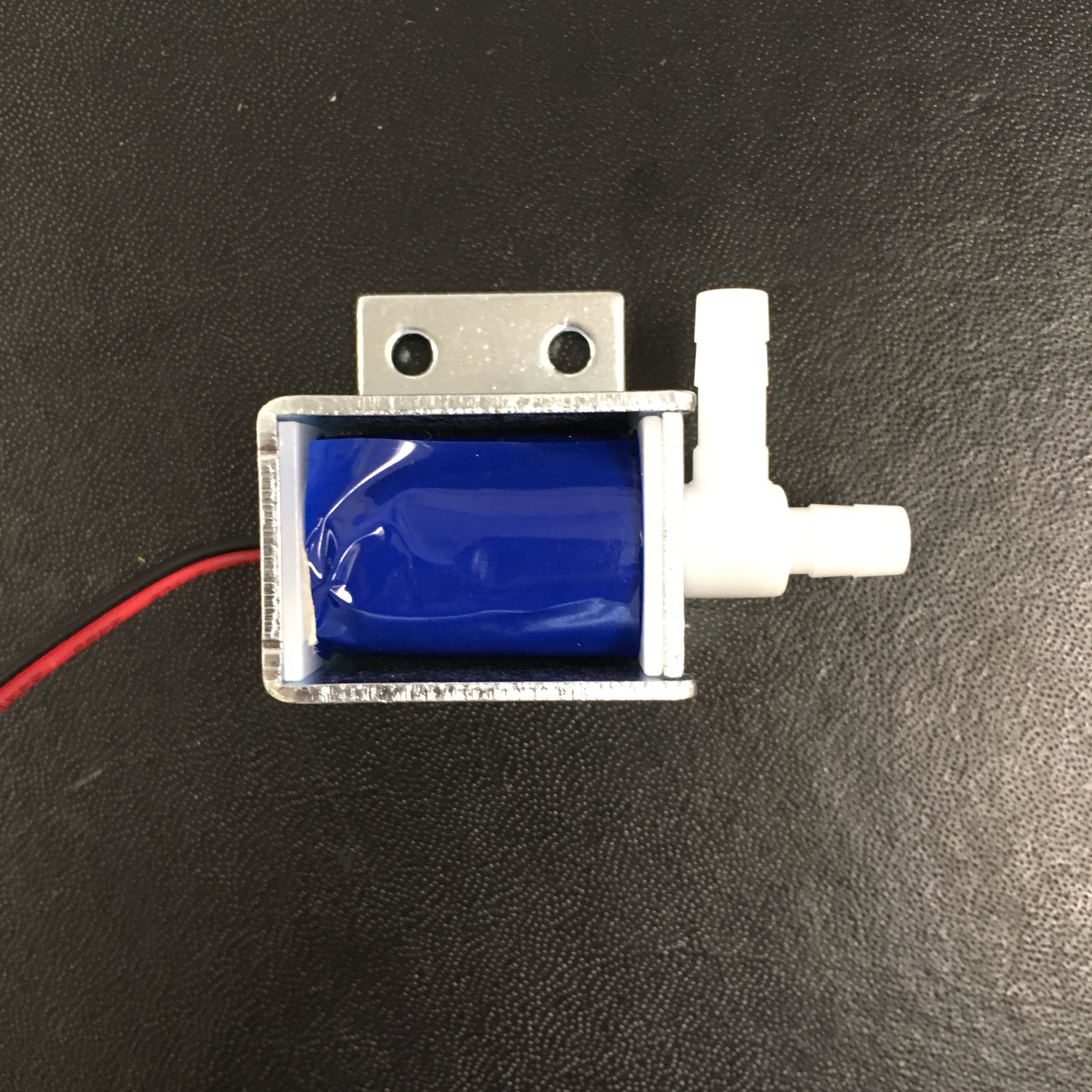
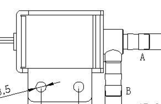
Solenoid valves open and close the flow of water with a linear actuator that pushes out or pulls in. In cheap normally-closed solenoids a spring holds the actuator out, pressing an o-ring against the face of the inlet as a seal. When current passes through the solenoid, the actuator pulls in against the spring and water is allowed to pass from inlet to outlet. The diagram below, taken from dyxminipumps.com, shows how our $1 valve’s inlet and outlet (openings A and B, respectively) are perpendicular to each other.
Using A as the inlet and B as the outlet, the valve will fail under quite low pressures. This is because the actuator is only blocking flow because of the force of the small spring; a small pressure from a pump only has to surpass the force of the spring to force the actuator backwards, opening flow from A to B. Orienting flow in the reverse direction, however, yields different results. Any pressure applied from opening B acts perpendicular to the motion of the actuator, neither adding nor subtracting from its closing force. In this orientation the valve will stay closed under very high pressures and a pressure buildup will cause other components of the water line failing first, such as the tubing popping out of fittings. This is quite undesirable in the normal application of these valves, such as in coffee machines, but we can take advantage of the failure behavior of the two orientations for the OPEnSampler.
By directing flow in the sample valves from B to A they will stay closed in the event of a pressure buildup, maintaining the integrity of the samples by preventing cross contamination. If the flush valve is oriented opposite, from A to B, it will be the weakest point in the water line and will fail first, effectively becoming a pressure relief valve for the system so that the water is released out the drain before fittings break.
This was tested in the lab by connecting the outlet of the pump directly to each of the valve’s openings in turn and running until failure. The pump ran for two minutes without valve failure while B was connected as the inlet and A the outlet, but failed after a few seconds in the A-B orientation.
Conclusion:
The sample valves will be oriented with flow from B to A and the flush valve will be oriented A to B. By taking advantage of the failure conditions of each orientation we can continue to use the cheap $1 valves without worrying about their low-pressure rating. This not only reduces further design work and prototyping but also saves about $150 per unit compared to the $7/piece alternative.


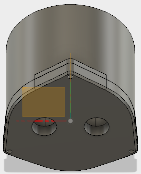


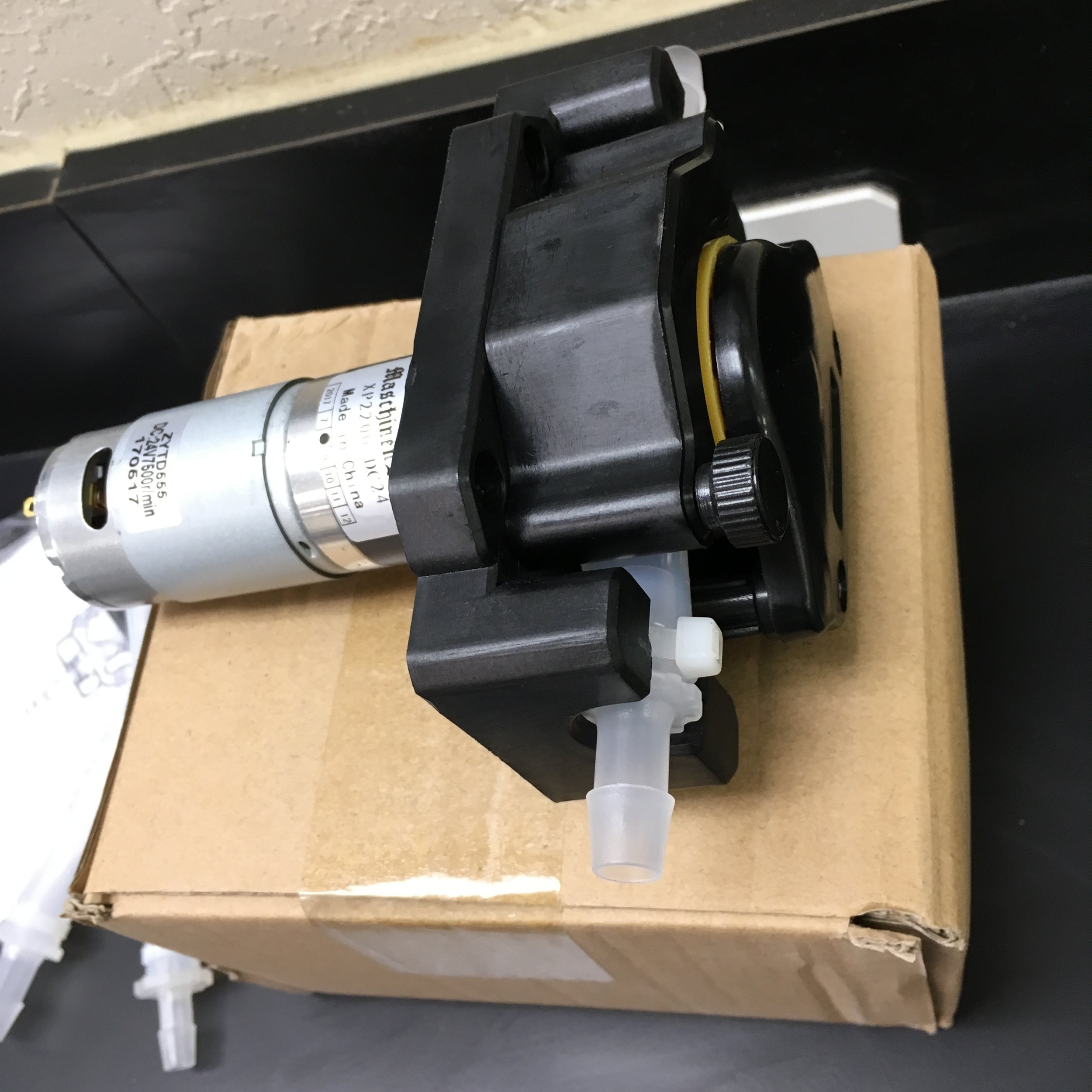
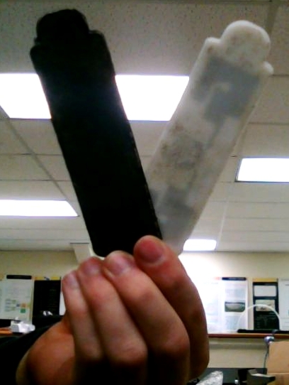

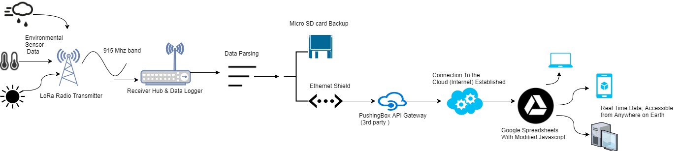

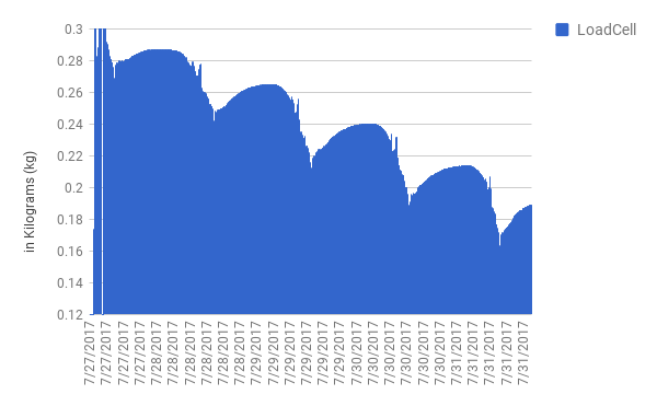
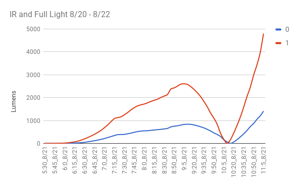
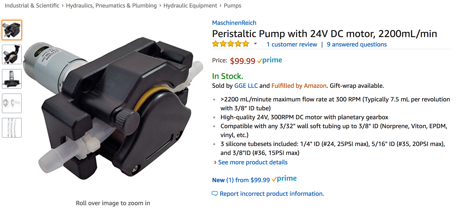
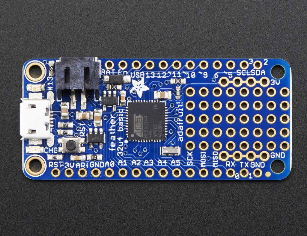
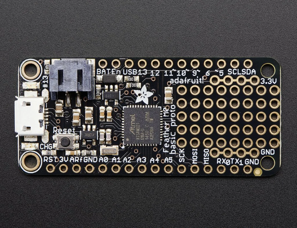
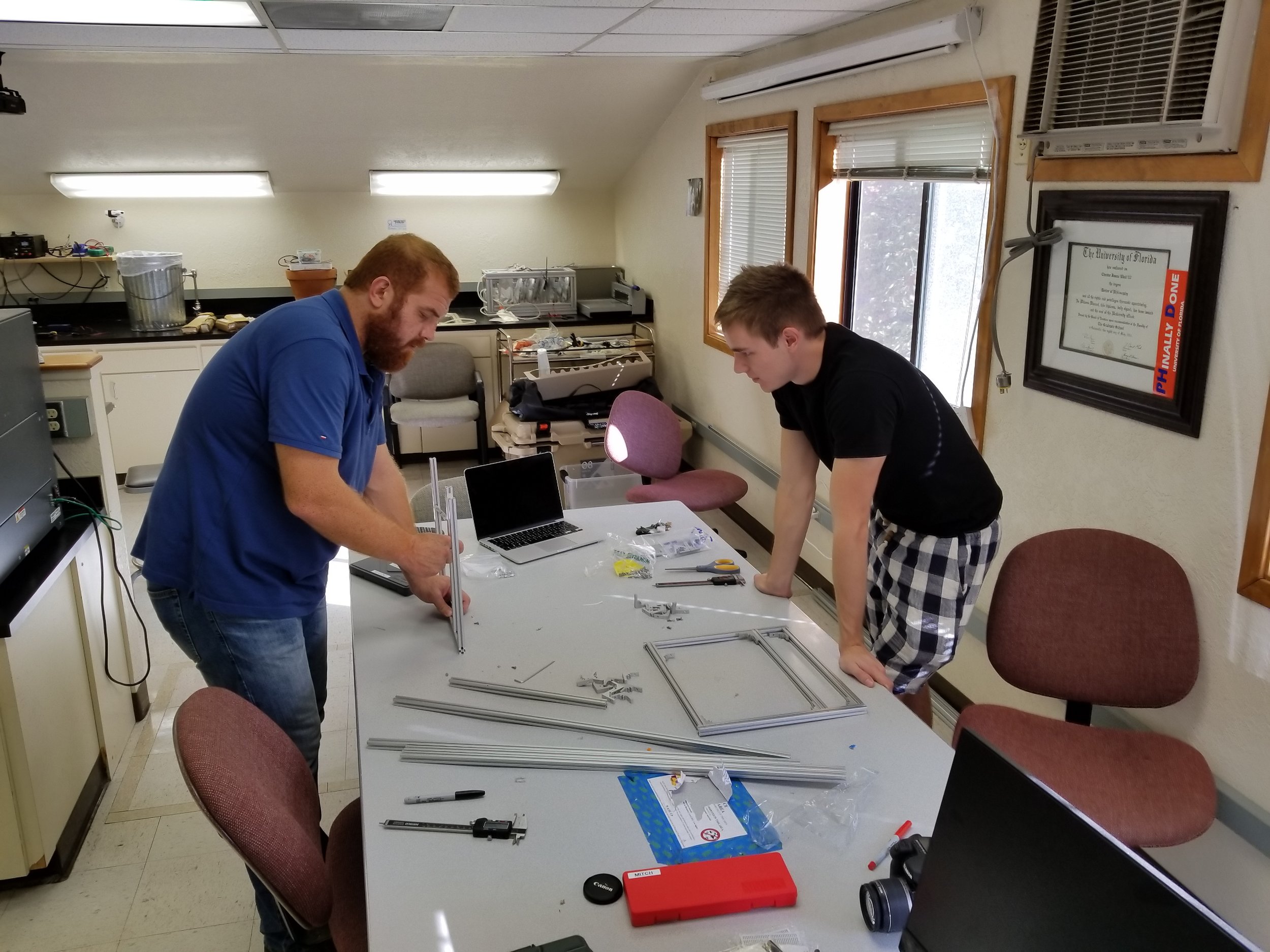

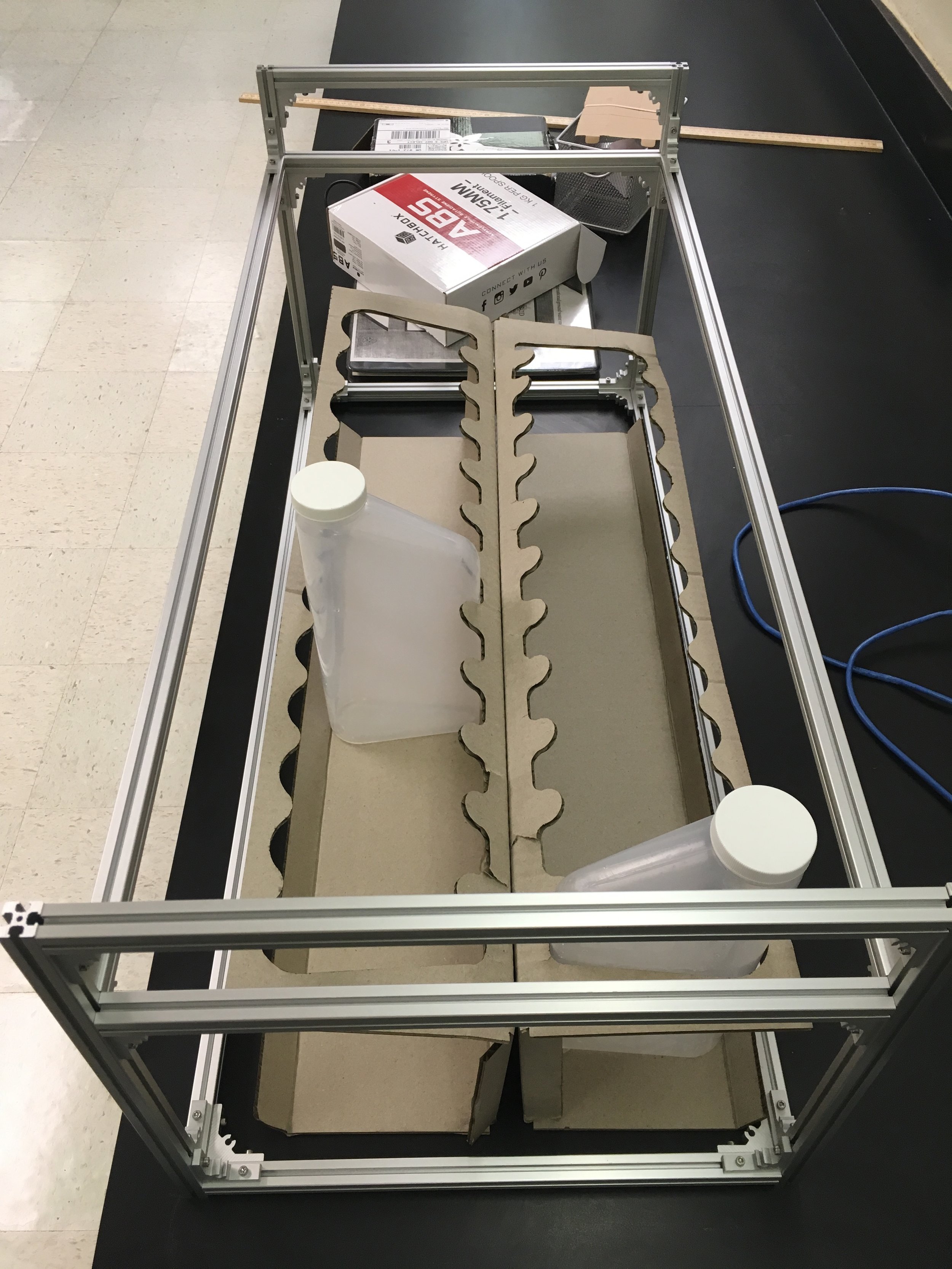
 Fig. 1.
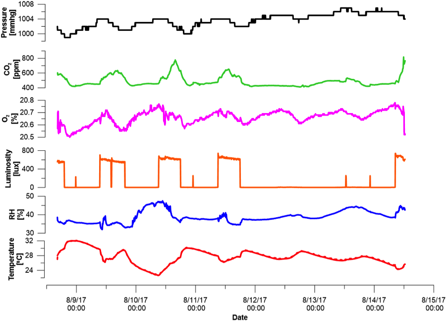 Fig. 2.
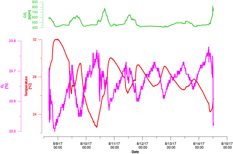 Fig. 3.
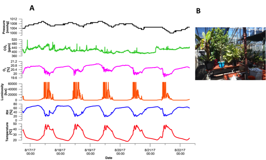 Fig. 4.
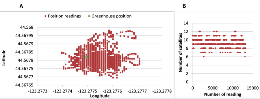 Fig. 5.